Lalgorithms - Nonparametric estimation of S-Shaped Functions with an application to Poverty Traps

Researchers are often interested in testing function shapes implied by theory. A notable example of such a function is an S-shaped one, which is initially convex on \([0, m_0]\) and subsequently concave on \([m_0, 1]\) (normalisation of support to \([0, 1]\) is wlog). Feng et al (2021) develop a nonparametric, tuning-free estimator of such functions using a primal-dual basis algorithm. Informally speaking, this method amounts to finding the threshold \(\hat{m}\) that minimises the MSE over the class of S-shaped functions on \([0, 1]\).

Poverty traps conjecture a S-shaped relationship between current income and future income: individuals or households below some threshold face a different set of constraints that results in them staying poor, while exceeding this threshold pulls them out of extreme poverty. This was experimentally tested in a large scale experiment by Balboni et al in Rural Bangladesh, who find evidence in favour of the S-shaped pattern characteristic of poverty traps.

Balboni et al use the nonparametric shape test proposed in Komorova and Hidalgo (2019) to test the null of global concavity. They then proceed to numerically solve for the poverty trap threshold using local polynomial regression. In this note, we revisit this exercise using the method proposed by Feng et al (2021) and find similar results.

library(LalRUtils)
libreq(Sshaped, ggExtra, ggplot2, rio, patchwork, np)

     wants       loaded
[1,] "Sshaped"   TRUE  
[2,] "ggExtra"   TRUE  
[3,] "ggplot2"   TRUE  
[4,] "rio"       TRUE  
[5,] "patchwork" TRUE  
[6,] "np"        TRUE

theme_set(lal_plot_theme())
root = "/home/alal/Desktop/00_Replications/BalboniEtAl2021_PovertyTraps"
df = import(file.path(root, "Data/PovertyTraps_analysis.dta")) %>% setDT

Exploratory Analysis

We first plot conditional expectations of asset levels immediately after the experiment as a function of baseline asset levels.

both_xc = df[survey_wave == 1 & stup == 1 & Lk1 <= 3]

p0 = ggplot(both_xc, aes(x = Lk0, y = Lk1, group = as.factor(treat),
      colour = as.factor(treat))) +
    geom_point() +
    geom_smooth(method = 'gam', alpha = 0.2) +
    scale_colour_brewer(palette = "Set1") + labs(colour = "treated")
ggMarginal(p0, type = "density", size = 7, groupColour = T, groupFill = T)

`geom_smooth()` using formula = 'y ~ s(x, bs = "cs")'
`geom_smooth()` using formula = 'y ~ s(x, bs = "cs")'

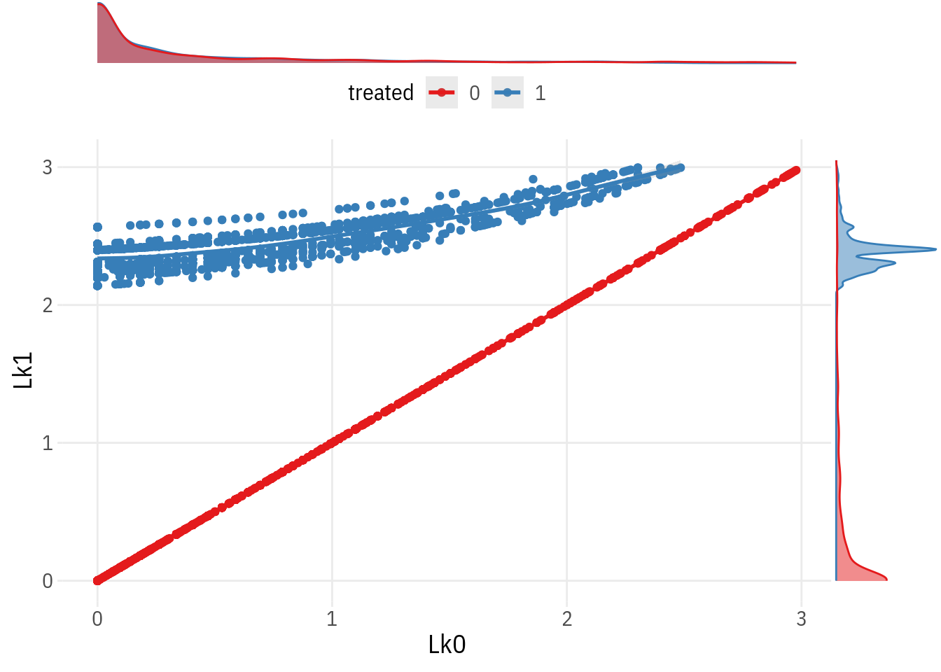
The treated group received a large positive shock to their income (since the experiment involved an asset transfer), while asset levels for control units remained unchanged.

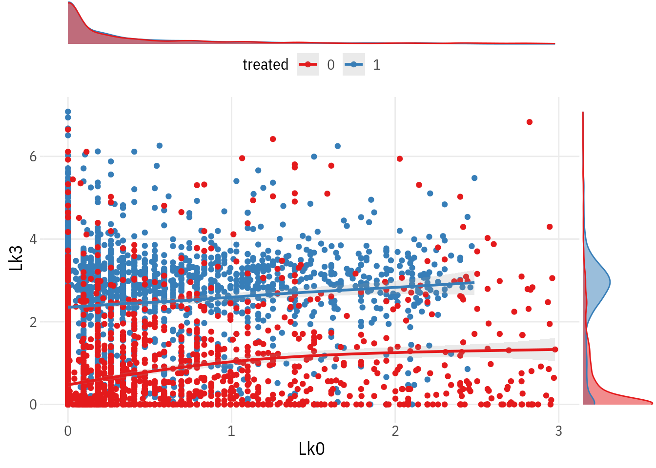
Next, we do the same for medium-run asset levels.

p1 = ggplot(both_xc, aes(x = Lk0, y = Lk3, group = as.factor(treat),
      colour = as.factor(treat))) +
    geom_point() +
    geom_smooth(method = 'gam', alpha = 0.2) +
    scale_colour_brewer(palette = "Set1") + labs(colour = "treated")
ggMarginal(p1, type = "density", size = 7, groupColour = T, groupFill = T)

`geom_smooth()` using formula = 'y ~ s(x, bs = "cs")'
`geom_smooth()` using formula = 'y ~ s(x, bs = "cs")'

This shows large positive, but highly heterogeneous effects.

Identifying the threshold

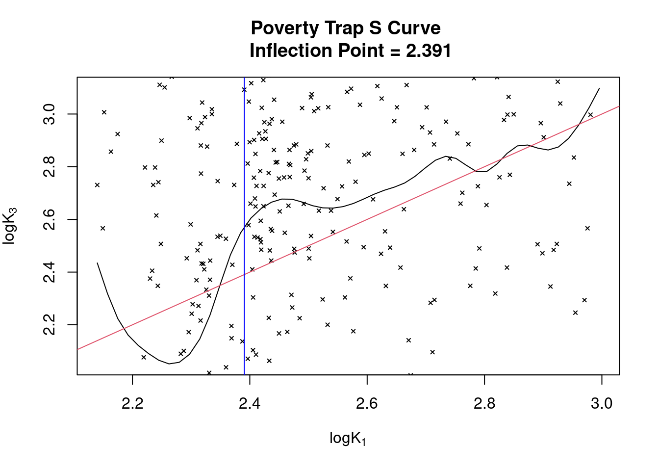
We compute the threshold using the Sshaped package developed by Feng et al. We restrict ourselves to the treatment group (since their crossing of the threshold is experimentally manipulated).

# nonparametric regression
m = npreg(bws = 0.04,  # computed beforehand
  txdat = as.vector(both_xc[treat==1, Lk1]),
  tydat = as.vector(both_xc[treat==1, Lk3]))

# dedupe grid for sshaped - average ys for each x
treated_obs = both_xc[treat == 1, .(Lk3 = mean(Lk3)), Lk1]
reg = sshapedreg(x = as.vector(treated_obs[['Lk1']]),
                 y = as.vector(treated_obs[['Lk3']]))

# final plot
plot(m, xlab=expression(logK[1]),ylab=expression(logK[3]),
  main = paste0("Poverty Trap S Curve \n Inflection Point = ", round(reg$inflection, 3))
  )
# points
points(treated_obs[['Lk1']], treated_obs[['Lk3']],
  pch = 4, cex = 0.5, type = "p",
  )
abline(a = 0, b = 1, col = 2)
lines(c(reg$inflection,reg$inflection),c(2,3.5),col="BLUE")

This gives us an inflection threshold of approximately 2.39, which is slighly larger than the 2.33 threshold computed by Balboni et al by numerically approximating the point where the nonparametric regression curve crosses the 45 degree line.