Causal inference with panel data can be viewed as a tensor completion problem, where the tensors in consideration are N \times T \times D, where N, T, and D are the number of units, periods, and treatment states respectively. WLOG, we focus on the binary case.
In most observational settings, treatment is rare and absorbing, so the \mathbf{Y}^(0) matrix is dense and \mathbf{Y}^{1} matrix is sparse. So, most researchers focus on the Average Treatment effect on the Treated (ATT), which is the difference {\mathbb{E}\left[Y^{1} - Y^0 | D = 1\right]}in the post-treatment periods for the treated units. Y^1s are observed for the treatment units {i: D = 1}, so the learning problem is to impute untreated potential outcomes Y^0.
Consider a N \times T outcome matrix of untreated potential outcomes \mathbf{Y}^0. Some subset N_1 units are treated from time T0+1 onwards. We can construct a corresponding matrix \mathbf{W}, which serves as a mask for \mathbf{Y}^0: whenever W_{it} is 1, \mathbf{Y}^0 is missing, and vice versa. The goal is to impute the missing entries corresponding with ? in the matrix below.
To impute missing potential outcomes, we may leverage
Vertical Regression: Learn the cross-sectional relationship between the outcomes for units in the pre-treatment period, assert that they are stable over time, and impute accordingly
Horizontal Regression: Learn the time-series relationship between pre-treatment and post-treatment outcomes for the never-treated units, assert that they are stable across units, and impute accordingly
Mixture: Mix between the two approaches.
Vertical Regression is particularly suitable when the data matrix is ‘fat’ (T >> N), while Horizontal Regression is particularly suitable when the data matrix is ‘thin’ (N >> T). MC is well suited for square-ish matrices.
1.1 Implementation
Code
root ="~/Desktop/0_computation_notes/metrics/00_CausalInference/Panel/"df =fread(file.path(root, "california_prop99.csv"))# custom function to construct wide outcome and treatment matrices from panel datasetup =panelMatrices(df, "State", "Year", "treated", "PacksPerCapita")attach(setup)mask =1- WYr =as.numeric(colnames(Y))# california seriesYcal = Y %>% .[nrow(.), ]
1.1.1 Difference in Differences
The difference in differences estimator can be thought of as a (naive) imputation estimator that constructs missing entries in \mathbf{Y}^0 as the average of nonmissing units + an intercept \mu, which is the average difference between treatment unit outcomes and control unit outcomes in the pre-treatment period. Note that this means all units get equal weight of 1/N_{co}, where N_{co} is the number of control units, and the weights aren’t data-driven.
Code
# diddid =DID(Y, mask) %>% .[nrow(.),]
Although the weights aren’t data driven, the offset \mu is learned on the basis of pre-treatment outcomes for treated and control units, so DiD may be considered a Vertical regression.
1.1.2 Synthetic Control
The Synthetic Control estimator imputes missing values in \mathbf{Y}^0 as a weighted average of post-treatment outcomes for control units, where the weights are learned using simplex regression of pre-treatment outcomes for the treatment unit on the pre-treatment outcomes of control units.
Code
# synthsyn =adh_mp_rows(Y, mask) %>% .[nrow(.),]
Synth is a Vertical regression.
1.1.3 Elastic Net Synthetic Control
The DIFP (Doudchenko-Imbens-Ferman-Pinto) estimator is similar to the synthetic control estimator but allows for negative weights and an intercept, and to this end uses ridge regression of pre-treatment outcomes for the treatment unit on the pre-treatment outcomes of control units to learn weights.
The time series approach involves regressing the post-treatment outcomes for never-treated units on pre-treatment outcomes, and using these coefficients to impute the untreated potential outcome for the treatment unit.
Here, the number of factors / rank R isn’t known and must be estimated. In applied econometric practice, researchers frequently use the additive fixed effects specification Y_{it}^0 = \gamma_i + \delta_t + \varepsilon_{it}, which is an instance of matrix completion with R = 2 where \mathbf{U} = [\boldsymbol{\alpha} \; ; 1] and \mathbf{V}^{\top}= [\mathbf{1} \; ; \boldsymbol{\delta}]. This factor structure can be considered in terms of the Singular Value Decomposition (SVD). Using the SVD of the observed data matrix \mathbf{Y}, we can write
where K = \min(M, N) and \mathbf{\Sigma} is a diagnonal K \times K matrix with sorted entries \sigma_1 \geq \sigma_2 \dots \sigma_k \geq 0. By the Eckart-Young Theorem, a low rank appoximation is found by truncating this expansion at rank R. This problem is, however, nonconvex. We can use an alternative matrix norm, the `nuclear’ norm, which is the sum of the singular values of \mathbf{L}. Letting \mathcal{O} denote nonmissing (i,t) pairs, we can write the optimization problem as
Matrix Completion is a mixed approach since it can leverage both vertical and horizontal information embedded in the low-rank approximation.
1.1.6 Singular Value Thresholding
Same as above, but nonconvex problem because the matrix rank is in the optimisation problem. Might scale poorly for large datasets, but inherits all qualities.
Code
# singular value thresholdingsvtY0 =fillY0(fill.SVT, lambda =5)
1.1.7 Nearest Neighbours Matching
Here, we find donors \mathcal{M} that match the pre-treatment outcomes for the treatment unit closely, and take the inverse-distance-weighted average to impute Y^0 in the post-period.
Code
# KNNknnY0 =fillY0(fill.KNNimpute, k =5)
This is a discretized version of Synth, so it is also Vertical.
Abadie, A., A. Diamond, and J. Hainmueller. (2010): “Synthetic Control Methods for Comparative Case Studies: Estimating the Effect of California’s Tobacco Control Program,” Journal of the American Statistical Association, 105, 493–505.
—. (2015): “Comparative Politics and the Synthetic Control Method,” American journal of political science, 59, 495–510.
Athey, S., M. Bayati, N. Doudchenko, G. Imbens, and K. Khosravi. (2017): “Matrix Completion Methods for Causal Panel Data Models,” arXiv [math.ST],.
Arkhangelsky, D., S. Athey, D. A. Hirshberg, G. W. Imbens, and S. Wager. (2021): “Synthetic Difference-in-Differences,” The American economic review,.
Bai, J. (2009): “Panel Data Models with Interactive Fixed Effects,” Econometrica: journal of the Econometric Society, 77, 1229–79.
Candès, E. J., & Tao, T. (2010). The power of convex relaxation: Near-optimal matrix completion. IEEE Transactions on Information Theory, 56(5), 2053-2080.
Doudchenko, N., and G. W. Imbens. (2016): “Balancing, Regression, Difference-In-Differences and Synthetic Control Methods: A Synthesis.,” Working Paper Series, National Bureau of Economic Research.
Gobillon, L., and T. Magnac. (2016): “Regional Policy Evaluation: Interactive Fixed Effects and Synthetic Controls,” The review of economics and statistics, 98, 535–51.
Mazumder, R., Hastie, T., & Tibshirani, R. (2010). Spectral regularization algorithms for learning large incomplete matrices. The Journal of Machine Learning Research, 11, 2287-2322.
Davenport, M. A., & Romberg, J. (2016). An overview of low-rank matrix recovery from incomplete observations. IEEE Journal of Selected Topics in Signal Processing, 10(4), 608-622.
Xu, Y. (2017): “Generalized Synthetic Control Method: Causal Inference with Interactive Fixed Effects Models,” Political analysis: an annual publication of the Methodology Section of the American Political Science Association, 25, 57–76.
Source Code
---title: Panel Data (DiD, Synth, MC) Causal Inferenceauthor: Apoorva Laldate: "2022-11-28"format: # pdf: # pdf-engine: xelatex # toc: true # number-sections: true # colorlinks: true # mainfont: TeX Gyre Pagella # monofont: Iosevka # highlight-style: github html: code-fold: true code-background: true code-overflow: wrap code-tools: true code-link: true highlight-style: arrow max-width: 1800px mainfont: IBM Plex Sans monofont: Iosevka number-sections: true html-math-method: katex fig-responsive: true colorlinks: true embed-resources: true df-print: pagedexecute: warning: false---::: {.hidden}$$% typographic\newcommand\Bigbr[1]{\left[ #1 \right ]}\newcommand\Bigcr[1]{\left\{ #1 \right \}}\newcommand\Bigpar[1]{\left( #1 \right )}\newcommand\Obr[2]{ \overbrace{#1}^{\text{#2}}}\newcommand\Realm[1]{\mathbb{R}^{#1}}\newcommand\Ubr[2]{\underbrace{#1}_{\text{#2}}}\newcommand\wb[1]{\overline{#1}}\newcommand\wh[1]{\widehat{#1}}\newcommand\wt[1]{\widetilde{#1}}\newcommand\Z{\mathbb{Z}}\newcommand\dd{\mathsf{d}}\DeclareMathOperator*{\argmin}{argmin}\DeclareMathOperator*{\argmax}{argmax}\newcommand\epsi{\varepsilon}\newcommand\phii{\varphi}\newcommand\tra{^{\top}}\newcommand\sumin{\sum_{i=1}^n}\newcommand\sumiN{\sum_{i=1}^n}\def\mbf#1{\mathbf{#1}}\def\mbi#1{\boldsymbol{#1}}\def\mrm#1{\mathrm{#1}}\def\ve#1{\mbi{#1}}\def\vee#1{\mathbf{#1}}\newcommand\R{\mathbb{R}}\newcommand\Ol[1]{\overline{#1}}\newcommand\SetB[1]{\left\{ #1 \right\}}\newcommand\Sett[1]{\mathcal{#1}}\newcommand\Str[1]{#1^{*}}\newcommand\Ul[1]{\underline{#1}}% stats\newcommand\Prob[1]{\mathbf{Pr}\left(#1\right)}\def\Exp#1{{\mathbb{E}\left[#1\right]}}\newcommand\var{\mathrm{Var}}\newcommand\Supp[1]{\text{Supp}\left[#1\right]}\newcommand\Var[1]{\mathbb{V}\left[#1\right]}\newcommand\Expt[2]{\mathbb{E}_{#1}\left[#2\right]}\newcommand\Covar[1]{\text{Cov}\left[#1\right]}\newcommand\Cdf[1]{\mathbb{F}\left(#1\right)}\newcommand\Cdff[2]{\mathbb{F}_{#1}\left(#2\right)}\newcommand\F{\mathsf{F}}\newcommand\ff{\mathsf{f}}\newcommand\Data{\mathcal{D}}\newcommand\Pdf[1]{\mathsf{f}\left(#1\right)}\newcommand\Pdff[2]{\mathsf{f}_{#1}\left(#2\right)}\newcommand\doo[1]{\Prob{Y |\,\mathsf{do} (#1) }}\newcommand\doyx{\Prob{Y \, |\,\mathsf{do} (X = x)}}% distributions\newcommand\Bern[1]{\mathsf{Bernoulli} \left( #1 \right )}\newcommand\BetaD[1]{\mathsf{Beta} \left( #1 \right )}\newcommand\Binom[1]{\mathsf{Bin} \left( #1 \right )}\newcommand\Diri[1]{\mathsf{Dir} \left( #1 \right )}\newcommand\Gdist[1]{\mathsf{Gamma} \left( #1 \right )}\newcommand\Normal[1]{\mathcal{N} \left( #1 \right )}\newcommand\Pois[1]{\mathsf{Poi} \left( #1 \right )}\newcommand\Unif[1]{\mathsf{U} \left[ #1 \right ]}% calc and linalg\newcommand\dydx[2]{\frac{\partial #1}{\partial #2}}\newcommand\Mat[1]{\mathbf{#1}}\newcommand\normm[1]{\lVert #1 \rVert}\newcommand\eucN[1]{\normm{#1}}\newcommand\pnorm[1]{\normm{#1}_p}\newcommand\lone[1]{\normm{#1}_1}\newcommand\ltwo[1]{\normm{#1}_2}\newcommand\lzero[1]{\normm{#1}_0}\newcommand\Indic[1]{\mathbb{1}_{#1}}$$:::# SetupCausal inference with panel data can be viewed as a tensor completion problem, where the tensors in consideration are $N \times T \times D$, where N, T, and D are the number of units, periods, and treatment states respectively.WLOG, we focus on the binary case.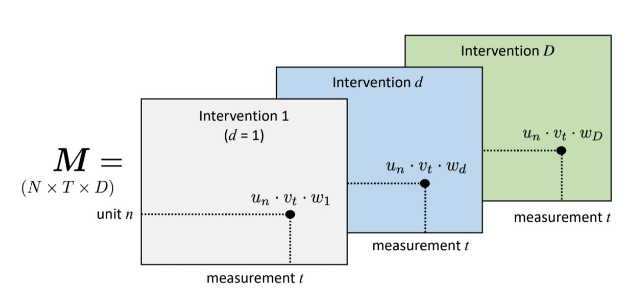In most observational settings, treatment is rare and absorbing, so the $\Mat{Y}^(0)$ matrix is dense and $\Mat{Y}^{1}$ matrix is sparse. So, most researchers focus on the Average Treatment effect on the Treated (ATT), which is the difference $\Exp{Y^{1} - Y^0 | D = 1}$ __in the post-treatment periods__ for the treated units. $Y^1$s are observed for the treatment units ${i: D = 1}$, so the learning problem is to impute untreated potential outcomes $Y^0$.Consider a $N \times T$ outcome matrix of untreated potential outcomes $\Mat{Y}^0$. Some subset $N_1$ units are treated from time $T0+1$ onwards. We can construct a corresponding matrix $\Mat{W}$, which serves as a mask for $\Mat{Y}^0$: whenever $W_{it}$ is 1, $\Mat{Y}^0$ is missing, and vice versa. The goal is to impute the missing entries corresponding with ? in the matrix below.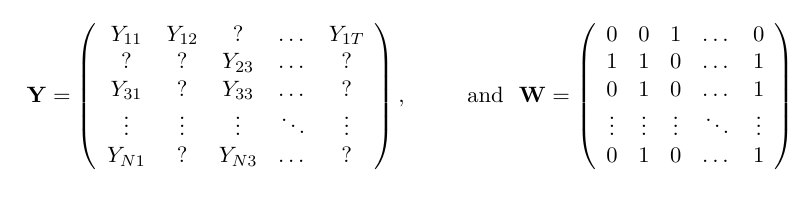To impute missing potential outcomes, we may leverage+ __Vertical Regression__: Learn the cross-sectional relationship between the outcomes for units in the pre-treatment period, assert that they are stable over time, and impute accordingly+ __Horizontal Regression__: Learn the time-series relationship between pre-treatment and post-treatment outcomes for the never-treated units, assert that they are stable across units, and impute accordingly+ __Mixture__: Mix between the two approaches.Vertical Regression is particularly suitable when the data matrix is 'fat' (T >> N),while Horizontal Regression is particularly suitable when the data matrix is 'thin' (N >> T). MC is well suited for square-ish matrices.```{r, echo = F, include = F}library(LalRUtils)libreq(magrittr, data.table, RColorBrewer, plotly, ggplot2, CVXR, MCPanel, filling)theme_set(lal_plot_theme())```## Implementation```{r}root ="~/Desktop/0_computation_notes/metrics/00_CausalInference/Panel/"df =fread(file.path(root, "california_prop99.csv"))# custom function to construct wide outcome and treatment matrices from panel datasetup =panelMatrices(df, "State", "Year", "treated", "PacksPerCapita")attach(setup)mask =1- WYr =as.numeric(colnames(Y))# california seriesYcal = Y %>% .[nrow(.), ]```### Difference in DifferencesThe difference in differences estimator can be thought of as a (naive) imputation estimator that constructs missing entries in $\Mat{Y}^0$ as the average of nonmissing units + an intercept $\mu$, which is the average difference between treatment unit outcomes and control unit outcomes in the pre-treatment period. Note that this means all units get equal weight of $1/N_{co}$, where $N_{co}$ is the number of control units, and the weights aren't data-driven.```{r}# diddid =DID(Y, mask) %>% .[nrow(.),]```Although the weights aren't data driven, the offset $\mu$ is learned on the basis of pre-treatment outcomes for treated and control units, so DiD may be considered a Vertical regression.### Synthetic ControlThe Synthetic Control estimator imputes missing values in $\Mat{Y}^0$ as a weighted average of post-treatment outcomes for control units, where the weights are learned using simplex regression of pre-treatment outcomes for the treatment unit on the pre-treatment outcomes of control units.```{r}# synthsyn =adh_mp_rows(Y, mask) %>% .[nrow(.),]```Synth is a Vertical regression.### Elastic Net Synthetic ControlThe DIFP (Doudchenko-Imbens-Ferman-Pinto) estimator is similar to the synthetic control estimator but allows for negative weights and an intercept, and to this end uses ridge regression of pre-treatment outcomes for the treatment unit on the pre-treatment outcomes of control units to learn weights.```{r}# enHenH =en_mp_rows(Y, mask, num_alpha =40) %>% .[nrow(.),]```EN Synth is a Vertical regression.### Elastic Net Time SeriesThe time series approach involves regressing the post-treatment outcomes for never-treated units on pre-treatment outcomes, and using these coefficients to impute the untreated potential outcome for the treatment unit.```{r}# enVenV =en_mp_rows(t(Y), t(mask), num_alpha =40) %>% .[, ncol(.)]```TS Synth is a Horizontal regression.### Matrix Completion with Nuclear Norm Minimization (M)The core idea of matrix completion in this setting is to model $\Mat{Y}^0$ as$$\Mat{Y}^{0} = \Mat{L}_{N \times T} + \ve{\epsi} = \Mat{U}_{N \times R} \Mat{V}\tra_{R \times T} + \ve{\epsi}_{N \times T}$$Here, the number of factors / rank $R$ isn't known and must be estimated.In applied econometric practice, researchers frequently use the additive fixed effects specification $Y_{it}^0 = \gamma_i + \delta_t + \epsi_{it}$, which is an instance of matrix completion with $R = 2$ where $\Mat{U} = [\ve{\alpha} \; ; 1]$ and $\Mat{V}\tra = [\vee{1} \; ; \ve{\delta}]$. This factor structure can be considered in terms of the Singular Value Decomposition (SVD). Using the SVD of the observed data matrix $\Mat{Y}$, we can write$$\Mat{Y}^0 = \Mat{U} \Mat{\Sigma} \Mat{V}\tra = \sum_{k=1}^K \sigma_k \vee{u}_k \vee{v}_k\tra$$where $K = \min(M, N)$ and $\Mat{\Sigma}$ is a diagnonal $K \times K$ matrix with sorted entries $\sigma_1 \geq \sigma_2 \dots \sigma_k \geq 0$. By the Eckart-Young Theorem, a low rank appoximation is found by truncating this expansion at rank $R$. This problem is, however, nonconvex. We can use an alternative matrix norm, the `nuclear' norm, which is the sum of the singular values of $\Mat{L}$. Letting $\Sett{O}$ denote nonmissing $(i,t)$ pairs, we can write the optimization problem as$$\text{min}_{\Mat{L}} \sum_{(i, t) \in \Sett{O}} \Bigpar{Y_{it} - L_{it}}^2 + \lambda_L \normm{\Mat{L}}_{*}$$where $\normm{\cdot}_{*}$ is the nuclear norm.```{r}# mcomco =mcnnm_cv(Y, mask) %>%predict_mc() %>% .[nrow(.),]```The same approach by hand without fixed effects.```{r}# filling package# fn for matrix completion libraryfillY0 = \(f, ...) f(Y0, ...)$X %>% .[nrow(.),]# mask treatment outcomes for filling packageY0 =replace(Y, !mask, NA)# nuclear norm - takes longnucY0 =fillY0(fill.nuclear)```Matrix Completion is a mixed approach since it can leverage both vertical and horizontal information embedded in the low-rank approximation.### Singular Value ThresholdingSame as above, but nonconvex problem because the matrix rank is in the optimisation problem. Might scale poorly for large datasets, but inherits all qualities.```{r}# singular value thresholdingsvtY0 =fillY0(fill.SVT, lambda =5)```### Nearest Neighbours MatchingHere, we find donors $\Sett{M}$ that match the pre-treatment outcomes for the treatment unit closely, and take the inverse-distance-weighted average to impute $Y^0$ in the post-period.```{r}# KNNknnY0 =fillY0(fill.KNNimpute, k =5)```This is a discretized version of Synth, so it is also Vertical.## Comparison```{r}predY =data.table(Yr, Ycal,`Nuclear Norm`= nucY0,`KNN`= knnY0,# `Simple Mean` = simY0,`Singular Value Thresholding`= svtY0,`Difference in Differences`= did,`Elastic Net H`= enH,`Elastic Net V`= enV,`Synth`= syn,`MCNNM`= mco) %>% setDTpredYlong =melt(predY, id.var ="Yr")fig =ggplot() +geom_line(data = df[State !="California"], aes(x = Year,y = PacksPerCapita, group = State),linewidth =0.5, alpha =0.1) +# californiageom_line(data = predYlong[variable =="Ycal"], aes(Yr, value), colour ='#060404',linewidth =2) +geom_vline(aes(xintercept =1988.5), col ='#44203c', linetype ='dotted') +# imputationsgeom_line(data = predYlong[variable !="Ycal"],aes(Yr, value, colour = variable), #height = 0, width = 0.5,linewidth =1.5, alpha =0.9) +scale_colour_brewer(palette ="Paired") +lal_plot_theme() +ylim(c(NA, 150)) +labs(colour ="")fig```Pre-treatment fit for DiD is bad, so it is likely over-estimated. Most other approaches produce roughly similar results.Interactive -- occasionally fails on quarto blog for some reason - see [here](https://gistcdn.githack.com/apoorvalal/981f11b05d50a35792f8d69741d7f7a3/raw/5940e07e8b5ebac111e5c84007c729f6c2f7fda0/index.html) for big friendly viz.```{r}htmlwidgets::saveWidget(ggplotly(fig), "CAtrajectories.html")ggplotly(fig)```## ReferencesAbadie, A., A. Diamond, and J. Hainmueller. (2010): “Synthetic Control Methods for Comparative Case Studies: Estimating the Effect of California’s Tobacco Control Program,” Journal of the American Statistical Association, 105, 493–505.---. (2015): “Comparative Politics and the Synthetic Control Method,” American journal of political science, 59, 495–510.Athey, S., M. Bayati, N. Doudchenko, G. Imbens, and K. Khosravi. (2017): “Matrix Completion Methods for Causal Panel Data Models,” arXiv [math.ST],.Arkhangelsky, D., S. Athey, D. A. Hirshberg, G. W. Imbens, and S. Wager. (2021): “Synthetic Difference-in-Differences,” The American economic review,.Bai, J. (2009): “Panel Data Models with Interactive Fixed Effects,” Econometrica: journal of the Econometric Society, 77, 1229–79.Candès, E. J., & Tao, T. (2010). The power of convex relaxation: Near-optimal matrix completion. IEEE Transactions on Information Theory, 56(5), 2053-2080.Doudchenko, N., and G. W. Imbens. (2016): “Balancing, Regression, Difference-In-Differences and Synthetic Control Methods: A Synthesis.,” Working Paper Series, National Bureau of Economic Research.Gobillon, L., and T. Magnac. (2016): “Regional Policy Evaluation: Interactive Fixed Effects and Synthetic Controls,” The review of economics and statistics, 98, 535–51.Mazumder, R., Hastie, T., & Tibshirani, R. (2010). Spectral regularization algorithms for learning large incomplete matrices. The Journal of Machine Learning Research, 11, 2287-2322.Davenport, M. A., & Romberg, J. (2016). An overview of low-rank matrix recovery from incomplete observations. IEEE Journal of Selected Topics in Signal Processing, 10(4), 608-622.Xu, Y. (2017): “Generalized Synthetic Control Method: Causal Inference with Interactive Fixed Effects Models,” Political analysis: an annual publication of the Methodology Section of the American Political Science Association, 25, 57–76.


