library(data.table)
#' Compute Neyman allocation propensity scores for inference-optimal treatment assignment in data table
#' @param df data.table
#' @param y outcome name
#' @param w treatment name
#' @param x covariate names (must all be discrete)
#' @return data.table with strata level conditional means, variances, propensity scores,
#'  and neyman allocation propensity scores.
#' @export
neymanAllocation = function(df, y, w, x){
    df1 = copy(df); N = nrow(df1)
    setnames(df1, c(y, w), c("y", "w"))
    nTreat = length(unique(df1$w))
    # conditional means and standard deviations within treat X covariate strata
    wxStrata = df1[, .(muHat = mean(y), sigHat = sd(y), num = .N), by = c(x, 'w')]
    # reshape to strata level
    wxStrataWide = dcast(wxStrata,
            as.formula(glue::glue("{glue::glue_collapse(x, '+' )} ~ w")),
            value.var = c("muHat", "sigHat", "num"))
    countCols = grep("num_", colnames(wxStrataWide), value = T)
    wxStrataWide[, nX := Reduce(`+`, .SD), .SDcols = countCols]
    wxStrataWide[, `:=`(fX = nX/N)]
    # empirical pscore
    nCols = grep("num_", colnames(wxStrataWide), value = T)
    wxStrataWide[, paste0("piHat_", nCols) := lapply(.SD, \(x) x/nX),
        .SDcols = nCols]
    # neyman allocation
    sigCols = grep("sigHat_", colnames(wxStrataWide), value = T)
    wxStrataWide[, sigDenom := Reduce(`+`, .SD), .SDcols = sigCols]
    wxStrataWide[, paste0("piNeyman_", nCols) := lapply(.SD, \(x) x/sigDenom ),
        .SDcols = sigCols]

    if(nTreat == 2){ # also returns treatment effects with 2 treatments; else compute desired contrasts yourself
        wxStrataWide[, tauX := muHat_1 - muHat_0]
        tau = wxStrataWide[, sum(fX * tauX)]
        se  = wxStrataWide[, sqrt(mean(sigHat_1^2/piHat_num_1 +
                                       sigHat_0^2/(1-piHat_num_0) +
                                       (tauX - tau)^2)) / sqrt(sum(nX))
                          ]
        return(list(strataLev = wxStrataWide, tau = tau, se = se))
    } else{
        return(wxStrataWide)
    }
}

#' Compute unconstrained optimal treatment probability
#' @param pNey neyman allocation propensity
#' @param p1 propensity score in first phase
#' @param kappa share of obs in first phase share
#' @return vector of variance-optimal treatment propensities
#' @export
ssProb = function(pNey, p1, kappa=.5){
    (1/(1 - kappa)) * (pNey - kappa * p1)
}The Feasible Neyman Allocation (Neyman 1934, Hahn, Hirano, Karlan (2011)) is an intuitive procedure to adaptively allocate treatment assignment in an experiment using the results from a pilot.
HHK propose a two-step approach to adaptive allocations to improve precision. WLOG, we focus on the two-arm case. Let \(X_i\) be a vector of discrete covariates, \(Y_i\) is the outcome, and \(A_i\) is a treatment indicator.
Hahn(1998) constructs the variance bound for the average treatment effect for binary treatments.
\[ V \geq \mathbb{E} \left[ \frac{\sigma_1^2}{p(X_i)} + \frac{\sigma_0^2}{1 - p(X_i)} + (\tau(X_i) - \tau)^2 \right] \]
Cattaneo(2010) derives the analogous bound for multiple discrete treatments. What follows applies for the general discrete treatments case as analyzed by Blackwell, Pashley, and Valentino.
With discrete covariates, the inverse propensity weighting using estimated propensity score attains this bound. Now, suppose we break the experiment into two phases: in the first phase, \(p(X) = \pi_1\) for all individuals. Next, we want to solve
\[ \text{min}_{p(\cdot)} \mathbb{E} \left[ \frac{\sigma_1^2}{p(X_i)} + \frac{\sigma_0^2}{1 - p(X_i)} + (\tau(X_i) - \tau)^2 \right] \]
In words, we want to choose a propensity score function to minimize the variance of the treatment effect estimate. This function is easily computable in closed form for discrete covariates.
To do this, we take the data from the first phase and estimate the empirical version of the variance bound, and then choose \(\hat{\pi}(x)\) to minimize it in the 2nd round. An interior solution satisfies the FOC
\[ \frac{\partial}{\partial \pi(x)} \left[ \frac{\hat{\sigma}_1^2 (x)}{\pi(x)} + \frac{\hat{\sigma}_0^2 (x)}{1 - \pi(x)} \right] = 0 \]
The solution is analytic and is given by the conditional standard deviation of the outcome in treatment cell k divided by the sum of the same across all arms. This is simplest to see when \(K = 2\).
\[ \pi(x) = \frac{\hat{\sigma}_1(x) }{\sum_{k=1}^{K} \hat{\sigma}_k(x) } \]
This is the solution for the overall sample. If the 2nd phase is to be analyzed independently, the above is the optimal propensity score. If the first and second phase are to be pooled, we solve for the second round propensity score
\[ \hat{\pi}_2(x) = \frac{1}{1-\kappa} [\pi(x) - \kappa \pi_1] \]
where \(\kappa = n_1/(n_1+n_2)\) is the share of observations in the first phase, and \(\pi_1\) is the propensity score in the first round (assumed but not required equal for all observations).
A constrained solution satisfying \(E[p(x)] = p\) for some \(p\) chosen by the implementer and can be solved for using numerical optimization [appendix A of HHR].
Application to (what else?) Lalonde.
data(lalonde.exp)
df = as.data.table(lalonde.exp)
y = 're78'; w = 'treat'
x = c("black", "nodegree", "u75")
kv = c(y, w, x)
df = df[, ..kv]

neymanAlloc = neymanAllocation(df, y, w, x)
neymanAlloc
$strataLev
black nodegree u75 muHat_0 muHat_1 sigHat_0 sigHat_1 num_0 num_1 nX fX
1: 0 0 0 7092 6381 6918 6005 4 6 10 0.02247
2: 0 0 1 11302 7229 3377 3156 4 5 9 0.02022
3: 0 1 0 8525 6905 6006 4444 11 8 19 0.04270
4: 0 1 1 5144 8766 4308 8690 26 10 36 0.08090
5: 1 0 0 4641 7725 7002 10353 14 17 31 0.06966
6: 1 0 1 3343 8798 3768 8795 21 26 47 0.10562
7: 1 1 0 4655 6787 6856 9965 53 43 96 0.21573
8: 1 1 1 3947 4362 4840 5375 127 70 197 0.44270
piHat_num_0 piHat_num_1 sigDenom piNeyman_num_0 piNeyman_num_1 tauX
1: 0.4000 0.6000 12923 0.5353 0.4647 -711.0
2: 0.4444 0.5556 6533 0.5169 0.4831 -4072.5
3: 0.5789 0.4211 10450 0.5748 0.4252 -1620.4
4: 0.7222 0.2778 12999 0.3314 0.6686 3621.3
5: 0.4516 0.5484 17355 0.4034 0.5966 3084.5
6: 0.4468 0.5532 12563 0.3000 0.7000 5455.4
7: 0.5521 0.4479 16822 0.4076 0.5924 2131.4
8: 0.6447 0.3553 10216 0.4738 0.5262 415.5
$tau
[1] 1560
$se
[1] 679.6neymanAlloc = neymanAlloc$strataLev
pscoreCols = grep("pi", colnames(neymanAlloc), value = T)
pscores = melt(neymanAlloc, id = x, measure = pscoreCols)
pscores = pscores[!(variable %like% "2ndStage")]
pscores[, c("type", "arm") := tstrsplit(variable, "_")[c(1, 3)]][, arm := as.numeric(arm)]
pscores[, type := ifelse(type == "piHat", "Current", "Optimal")]
pscores[, xstratum := do.call(paste, c(.SD, sep = "_")),
.SDcols = c("black", "nodegree", "u75")]library(ggplot2)
ggplot(pscores, aes(x = as.factor(arm), y = value, colour = type)) +
geom_point() +
facet_wrap(~ xstratum) +
lal_plot_theme() +
labs(title = "Propensity Scores", subtitle = "Current versus Optimal by Covariate bin")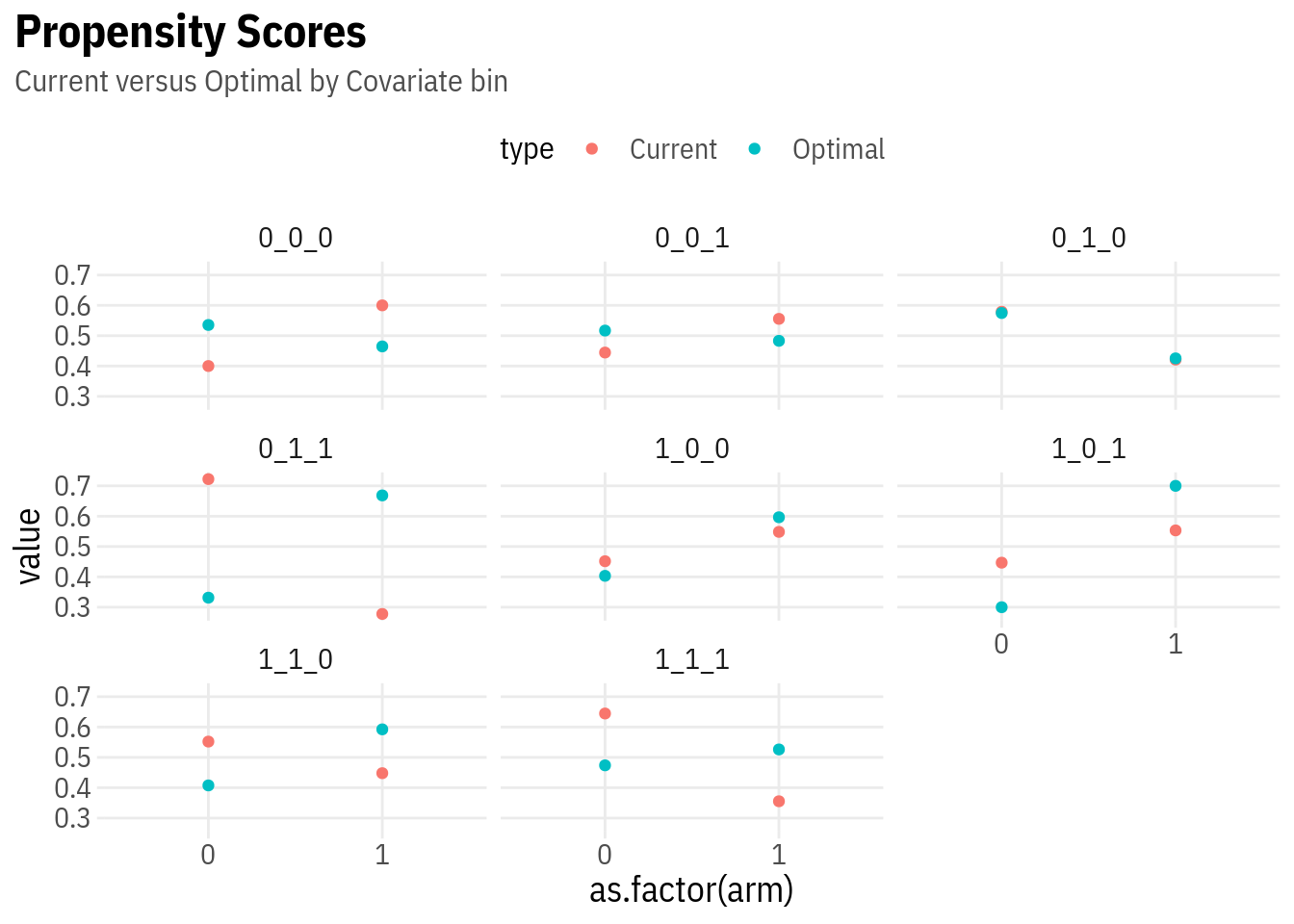
Vertical distance between the two dots indicates the magnitude of propensity score changes in the second round, which can be computed for a given value of \(\kappa\).
Let us now pretend that we want to run a 2nd phase that is 4x the size. Then, the optimal propensities can be computed using ssProb, which takes baseline propensity, Neyman propensity, and the share of observations in the pilot.
# 2nd stage optimal probability
neymanAlloc[, pi1_2ndStage := ssProb(piNeyman_num_1, piHat_num_1, kappa = 0.2)]
neymanAlloc
black nodegree u75 muHat_0 muHat_1 sigHat_0 sigHat_1 num_0 num_1 nX fX
1: 0 0 0 7092 6381 6918 6005 4 6 10 0.02247
2: 0 0 1 11302 7229 3377 3156 4 5 9 0.02022
3: 0 1 0 8525 6905 6006 4444 11 8 19 0.04270
4: 0 1 1 5144 8766 4308 8690 26 10 36 0.08090
5: 1 0 0 4641 7725 7002 10353 14 17 31 0.06966
6: 1 0 1 3343 8798 3768 8795 21 26 47 0.10562
7: 1 1 0 4655 6787 6856 9965 53 43 96 0.21573
8: 1 1 1 3947 4362 4840 5375 127 70 197 0.44270
piHat_num_0 piHat_num_1 sigDenom piNeyman_num_0 piNeyman_num_1 tauX
1: 0.4000 0.6000 12923 0.5353 0.4647 -711.0
2: 0.4444 0.5556 6533 0.5169 0.4831 -4072.5
3: 0.5789 0.4211 10450 0.5748 0.4252 -1620.4
4: 0.7222 0.2778 12999 0.3314 0.6686 3621.3
5: 0.4516 0.5484 17355 0.4034 0.5966 3084.5
6: 0.4468 0.5532 12563 0.3000 0.7000 5455.4
7: 0.5521 0.4479 16822 0.4076 0.5924 2131.4
8: 0.6447 0.3553 10216 0.4738 0.5262 415.5
pi1_2ndStage
1: 0.4308
2: 0.4650
3: 0.4263
4: 0.7662
5: 0.6086
6: 0.7368
7: 0.6285
8: 0.5689these are different from the baseline propensity of \(0.4\).
Finally, the standard error can be computed as
\[ \begin{gathered} S E=\frac{1}{\sqrt{n}} \sqrt{\frac{1}{n} \sum_{i=1}^{n}\left(\frac{\widehat{\sigma}_{1}^{2}\left(X_{i}\right)}{\pi\left(X_{i}\right)}+\frac{\widehat{\sigma}_{0}^{2}\left(X_{i}\right)}{1-\pi\left(X_{i}\right)}+\left(\widehat{\beta}\left(X_{i}\right)-\widehat{\beta}\right)^{2}\right)} \\ \widehat{\beta}(x)=\frac{\frac{\sum_{i=1}^{n} W_{i} Y_{i} 1\left(X_{i}=x\right)}{\sum_{i=1}^{n} 1\left(X_{i}=x\right)}}{\widehat{p}(x)}-\frac{\frac{\sum_{i=1}^{n}\left(1-W_{i}\right) Y_{i} 1\left(X_{i}=x\right)}{\sum_{i=1}^{n} 1\left(X_{i}=x\right)}}{1-\widehat{p}(x)} \end{gathered} \]
This also generalizes to multiple treatments (where the gains from adaptivity are particularly strong) using the efficiency bounds in Cattaneo (2010).