Jeff Wooldridge recently posted about different estimators for treatment effects under unconfoundedness, and in particular emphasized a somewhat overlooked Regression Adjustment with inverse propensity weights method, which can be viewed as a (simple) instantiation of the Targeted Maximum Likelihood (TMLE) approach to estimation under unconfoundedness.

Exposition from Imbens (2004)

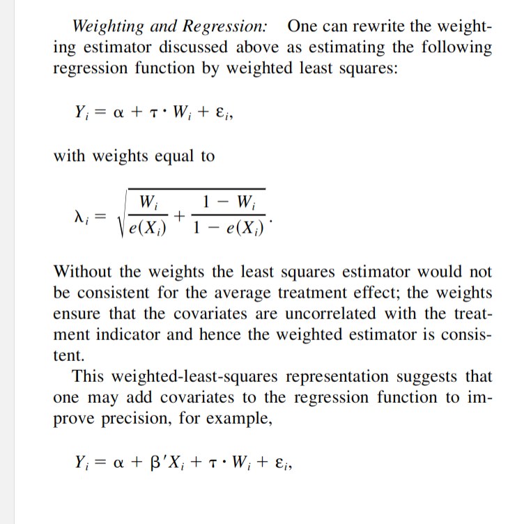
Here, we implement and benchmark some of these estimators and study their behaviour under different forms of mis-specification, and conclude that IPWRA generally works pretty well. It is effectively quite similar to entropy balancing weights in terms of bias and variance, which are also doubly robust in that they implicitly fit a linear model and logistic propensity score.

import numpy as np
import pandas as pd
from econml.dr import LinearDRLearner
from joblib import Parallel, delayed
from lightgbm import LGBMClassifier, LGBMRegressor
from sklearn.linear_model import LinearRegression, LogisticRegression
import empirical_calibration as ec

import scipy
from typing import List

utils

DGP to generate a dataframe generated from a user-supplied pscore, outcome, and heterogeneous effects function.

# %%  DGP
def binary_dgp(n, k, pscore_fn, tau_fn, outcome_fn, k_cat=1):
    Sigma = np.random.uniform(-1, 1, (k, k))
    Sigma = Sigma @ Sigma.T
    Xnum = np.random.multivariate_normal(np.zeros(k), Sigma, n)
    # generate categorical variables
    Xcat = np.random.binomial(1, 0.5, (n, k_cat))
    X = np.c_[Xnum, Xcat]
    W = np.random.binomial(1, pscore_fn(X), n).astype(int)
    Y = outcome_fn(X, W, tau_fn)
    df = pd.DataFrame(
        np.c_[Y, W, X], columns=["Y", "W"] + [f"X{i}" for i in range(k + 1)]
    )
    return df

def sim_summariser(dat, truth=1):
    return {
        "bias": np.mean(dat, axis=0) - truth,
        "var": np.var(dat, axis=0),
        "rmse": np.sqrt(np.mean((dat - truth) ** 2, axis=0)),
    }

Regression Adjustment + IPW

Omnibus function to compute Regression Adjustment, IPW, and IPW-RA. This is now available in aipyw.

from sklearn.preprocessing import StandardScaler

def ipwra(
    y: np.ndarray,
    w: np.ndarray,
    X: np.ndarray,
    estimand: str = "ATE",
    typ: str = "both",
):
    # standardize X
    sca = StandardScaler()
    Xtilde = sca.fit_transform(X)
    # weight specification
    if typ in ["both", "ipw"]:
        lr = LogisticRegression(
            C=1e12
        )  # make inverse reg strength big for no regularisation
        lr.fit(X, w)
        p = lr.predict_proba(X)  # returns (1-e(x), e(x))
        if estimand == "ATE":
            wt = w / p[:, 1] + (1 - w) / p[:, 0]
        elif estimand == "ATT":
            rho = np.mean(w)
            wt = p[:, 1] / rho + (1 - w) / p[:, 0]
    # covariate matrix specification
    if typ in ["both", "ra"]:
        XX = np.c_[
            np.ones(len(w)), w, Xtilde, w[:, np.newaxis] * Xtilde
        ]  # design matrix has [1, W, X, W * X] where X is centered
    else:
        XX = np.c_[np.ones(len(w)), w]  # pure IPW
    if typ == "ra":
        wt = None
    return LinearRegression().fit(XX, y, sample_weight=wt).coef_[1]  # w coef

edit: an earlier version manually applied np.sqrt to the weights, which LinearRegression does internally. Τhis was incorrect and has been fixed.

User-facing instantiation that accepts a dataframe, and computes bootstrap confidence intervals by default.

def bootstrap_ipwra(
    df: pd.DataFrame,
    outcome: str = "Y",
    treatment: str = "W",
    covariates: List = [],
    typ: str = "both",
    alpha: float = 0.05,
    n_iterations: int = 100,
    n_jobs: int = -1,
):
    if len(covariates) == 0:  # use all remaining columns as covariates
        covariates = df.columns.difference([outcome, treatment]).tolist()
    point_estimate = ipwra(df[outcome].values, df[treatment].values, df[covariates].values, typ=typ)
    if n_iterations == 0:
        return {"est": point_estimate.round(4)}

    def onerep():
        bsamp = df.sample(n=len(df), replace=True)
        return ipwra(bsamp[outcome].values, bsamp[treatment].values, bsamp[covariates].values, typ=typ)

    # multi-thread bootstrap
    replicates = Parallel(n_jobs=n_jobs)(delayed(onerep)() for _ in range(n_iterations))
    replicates = np.array(replicates)
    lb, ub = np.percentile(replicates, [alpha / 2 * 100, (1 - alpha / 2) * 100])
    return {
        "est": point_estimate.round(4),
        f"{(1-alpha)*100}% CI (Bootstrap)": np.r_[lb, ub].round(4),
    }

Example of use:

def outcome_fn(x, w, taufn):
    base_term = x[:, 0] + 2 * x[:, 1] + x[:, 3]
    return taufn(x) * w + base_term + np.random.normal(0, 1, len(w))


def pscore_fn(x):
    lin = x[:, 0] - x[:, 1] - x[:, 2] + x[:, 3] + np.random.normal(0, 1, x.shape[0])
    return scipy.special.expit(lin)


df = binary_dgp(n = 10_000, k = 4, tau_fn = lambda x: 1,
    pscore_fn = pscore_fn, outcome_fn = outcome_fn)
df.head()

	Y	W	X0	X1	X2	X3	X4
0	0.853669	1.0	0.540357	-0.246628	-1.208470	-2.053303	1.0
1	-2.828752	0.0	0.055509	-0.042991	-0.779749	-1.748115	1.0
2	-2.055299	1.0	0.288326	-1.199592	-0.606765	-1.226635	1.0
3	3.797470	0.0	-0.708268	1.232548	1.141870	1.584794	0.0
4	1.116264	1.0	0.317727	-0.945817	-0.163137	1.769615	1.0

# default args conform to simulated data; else supply variable names
bootstrap_ipwra(df)

{'est': 0.9953, '95.0% CI (Bootstrap)': array([0.9357, 1.0547])}

Simulations

Our simulation machine accepts DGP parameters and returns a list of estimates. For the first 3 estimators, we use linear + logistic specifications that accommodate linear and logistic propensity scores, so any non-linearity generates misspecification. The last AIPW estimator uses boosting regression and classification and should (at slow rates) learn all functions, so will never be misspecified.

def onesim(**kwargs):
    df = binary_dgp(**kwargs)
    outcome_column, treatment_column = "Y", "W"
    feature_columns = df.columns.difference([outcome_column, treatment_column]).tolist()
    # naive
    naive = df.groupby("W")["Y"].mean().diff()[1] # treat - ctrl
    # ipw and ipwra
    ra, ipw, ipwra = (
        bootstrap_ipwra(df, n_iterations=0, typ="ra"),
        bootstrap_ipwra(df, n_iterations=0, typ="ipw"),
        bootstrap_ipwra(df, n_iterations=0, typ="both"),
    )
    # aipw
    m = LinearDRLearner(
        model_regression=LGBMRegressor(n_estimators=50, verbose=-1),
        model_propensity=LGBMClassifier(n_estimators=50, verbose=-1),
    )
    m.fit(
        Y=df["Y"],
        T=df["W"],
        W=df[feature_columns],
    )
    dml_est = m.ate_inference().mean_point
    # balancing weights
    qweights, _ = ec.maybe_exact_calibrate(
                                covariates=df.query("W==0")[feature_columns].values,
                                target_covariates=df.query("W==1")[feature_columns].values,
                                objective=ec.Objective.QUADRATIC,
                                )
    eweights, _ = ec.maybe_exact_calibrate(
                                covariates=df.query("W==0")[feature_columns].values,
                                target_covariates=df.query("W==1")[feature_columns].values,
                                objective=ec.Objective.ENTROPY,
                                )
    qb_est = df.query("W==1")["Y"].mean() - np.average(df.query("W==0")["Y"], weights=qweights)
    eb_est = df.query("W==1")["Y"].mean() - np.average(df.query("W==0")["Y"], weights=eweights)

    return np.r_[naive, ra["est"], ipw["est"], ipwra["est"], dml_est, qb_est, eb_est]

tau_fn = lambda x: 1
n, k, nsim = 10_000, 3, 100
estimators = ['naive', 'ra', 'ipw', 'ipwra', 'aipw', 'qb', 'eb']

both correctly specified

Linear outcome and logistic pscore.

def outcome_fn(x, w, taufn):
    base_term = x[:, 0] + 2 * x[:, 1] + x[:, 3]
    return taufn(x) * w + base_term + np.random.normal(0, 1, len(w))


def pscore_fn(x):
    lin = x[:, 0] - x[:, 1] - x[:, 2] + x[:, 3] + np.random.normal(0, 1, x.shape[0])
    return scipy.special.expit(lin)

onesim(n=n, k=k, pscore_fn=pscore_fn, tau_fn=tau_fn, outcome_fn=outcome_fn)

array([-0.37865908,  1.0071    ,  0.9765    ,  0.9991    ,  1.02255154,
        0.9882471 ,  0.98856997])

linear_sims = np.array(
    Parallel(n_jobs=-1)(
        delayed(onesim)(
            n=n, k=k, pscore_fn=pscore_fn, tau_fn=tau_fn, outcome_fn=outcome_fn
        )
        for _ in range(nsim)
    )
)
linear_summary = sim_summariser(linear_sims)
pd.DataFrame.from_dict(linear_summary).set_axis(estimators)

	bias	var	rmse
naive	-0.333937	1.189322	1.140542
ra	-0.000373	0.000628	0.025067
ipw	-0.006068	0.005668	0.075530
ipwra	-0.003223	0.000829	0.028967
aipw	0.011722	0.001381	0.038965
qb	-0.003911	0.000931	0.030758
eb	-0.005386	0.001297	0.036418

good weights don’t add much variance to IPWRA (over RA). IPW is quite bad even though the model is correctly specified.

correct outcome, incorrect propensity

introduce nonlinearity into the pscore.

def outcome_fn(x, w, taufn):
    base_term = x[:, 0] + 2 * x[:, 1] + x[:, 3]
    return taufn(x) * w + base_term + np.random.normal(0, 1, len(w))


def pscore_fn(x):
    lin = (
        -x[:, 0]
        - x[:, 1]
        - x[:, 2]
        + x[:, 3]
        + np.exp(x[:, 3])
        + x[:, 2] ** 2
        + 0.1 * x[:, 1] ** 3
        + x[:, 0] * x[:, 1]
        + np.random.normal(0, 1, x.shape[0])
    )
    return scipy.special.expit(lin)


nlinear_sims1 = np.array(
    Parallel(n_jobs=12)(
        delayed(onesim)(
            n=n, k=k, pscore_fn=pscore_fn, tau_fn=tau_fn, outcome_fn=outcome_fn
        )
        for _ in range(nsim)
    )
)
nlinear_summary1 = sim_summariser(nlinear_sims1)
pd.DataFrame.from_dict(nlinear_summary1).set_axis(estimators)

	bias	var	rmse
naive	-0.391805	0.367960	0.722130
ra	0.004664	0.001873	0.043533
ipw	-0.375230	0.146017	0.535551
ipwra	0.000944	0.002958	0.054398
aipw	0.059299	0.035076	0.196450
qb	0.002870	0.003020	0.055026
eb	-0.001717	0.004221	0.064991

Bad pscore does not hurt IPWRA in terms of bias, but increases variance a bit.

incorrect outcome, correct propensity

introduce non-linearity into the outcome model.

def outcome_fn(x, w, taufn):
    base_term = (
        x[:, 0]
        + 2 * x[:, 1]
        + x[:, 3]
        + np.exp(x[:, 0])
        + 2 * (x[:, 1] > 0.5)
        + x[:, 1] ** 2
        + np.sqrt(np.abs(x[:, 2]))
        + x[:, 0] * x[:, 2]
    )
    return taufn(x) * w + base_term + np.random.normal(0, 1, len(w))


def pscore_fn(x):
    lin = (
        -x[:, 0]
        - x[:, 1]
        - x[:, 2]
        + x[:, 3]
        + np.random.normal(0, 1, x.shape[0])
    )
    return scipy.special.expit(lin)


nlinear_sims2 = np.array(
    Parallel(n_jobs=12)(
        delayed(onesim)(
            n=n, k=k, pscore_fn=pscore_fn, tau_fn=tau_fn, outcome_fn=outcome_fn
        )
        for _ in range(nsim)
    )
)
nlinear_summary2 = sim_summariser(nlinear_sims2)
pd.DataFrame.from_dict(nlinear_summary2).set_axis(estimators)

	bias	var	rmse
naive	-2.913566	4.837368	3.650512
ra	0.328193	0.246748	0.595365
ipw	-0.065889	0.107900	0.335024
ipwra	0.050050	0.036513	0.197530
aipw	-0.033077	0.073476	0.273075
qb	0.494620	0.102425	0.589129
eb	0.092074	0.030125	0.196477

RA has some bias. IPWRA has lower bias, which suggests that the weights help a bit.

both incorrect

both outcome and propensity have non-linearity.

def outcome_fn(x, w, taufn):
    base_term = (
        x[:, 0]
        + 2 * x[:, 1]
        + x[:, 3]
        + np.exp(x[:, 0])
        + 2 * (x[:, 1] > 0.5)
        + x[:, 1] ** 2
        + np.sqrt(np.abs(x[:, 2]))
        + x[:, 0] * x[:, 2]
    )
    return taufn(x) * w + base_term + np.random.normal(0, 1, len(w))


def pscore_fn(x):
    lin = (
        x[:, 0]
        - x[:, 1]
        - x[:, 2]
        + x[:, 3]
        + np.exp(x[:, 3])
        + x[:, 2] ** 2
        + 0.1 * x[:, 1] ** 3
        + x[:, 0] * x[:, 1]
        + np.random.normal(0, 1, x.shape[0])
    )
    return scipy.special.expit(lin)


nlinear_sims3 = np.array(
    Parallel(n_jobs=12)(
        delayed(onesim)(
            n=n, k=k, pscore_fn=pscore_fn, tau_fn=tau_fn, outcome_fn=outcome_fn
        )
        for _ in range(nsim)
    )
)
nlinear_summary3 = sim_summariser(nlinear_sims3)
pd.DataFrame.from_dict(nlinear_summary3).set_axis(estimators)

	bias	var	rmse
naive	0.769820	2.343603	1.713542
ra	0.058784	3.701395	1.924799
ipw	-4.453326	128.446402	12.176967
ipwra	0.441008	7.651208	2.801017
aipw	0.059865	0.040356	0.209618
qb	-0.392092	5.627199	2.404357
eb	-1.021150	10.837197	3.446729

All bets are off, only AIPW with boosting nuisances works well.