In [18]:
rm(list = ls())
library(LalRUtils)
libreq(data.table, magrittr, tidyverse, janitor, stargazer2,
       knitr, IRdisplay, np)
theme_set(lal_plot_theme_d())
set.seed(42)
options(repr.plot.width = 10, repr.plot.height=7)
chr = function(...) as.character(...)
#%%
Continuous Outcome
In [56]:
data("cps71")
cps71 %>% glimpse
In [60]:
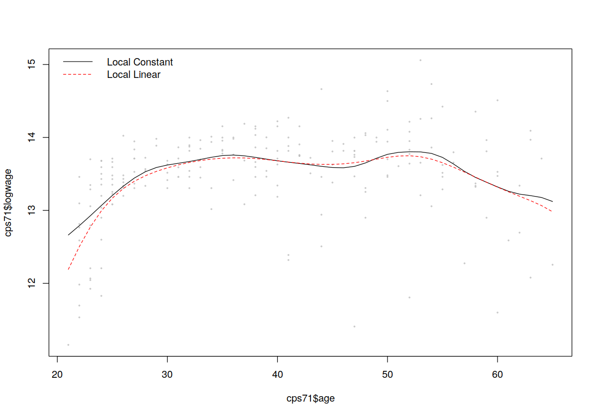
plot(cps71$age,cps71$logwage,cex=0.25,col="grey")
## Fit a (default) local constant model (since we do not explicitly
## call npregbw() which conducts least-squares cross-validated
## bandwidth selection by default it is automatically invoked when we
## call npreg())
model.lc <- npreg(logwage~age, data = cps71)
## Plot the fitted values (the colors and linetypes allow us to
## distinguish different plots on the same figure)
lines(cps71$age,fitted(model.lc),col=1,lty=1)
## Fit a local linear model (we use the arguments regtype="ll" to do
## this)
model.ll <- npreg(logwage~age,regtype="ll", cps71)
## Plot the fitted values with a different color and linetype
lines(cps71$age,fitted(model.ll),col=2,lty=2)
## Add a legend
legend("topleft",
       c("Local Constant","Local Linear"),
       lty=c(1,2),
       col=c(1,2),
       bty="n")
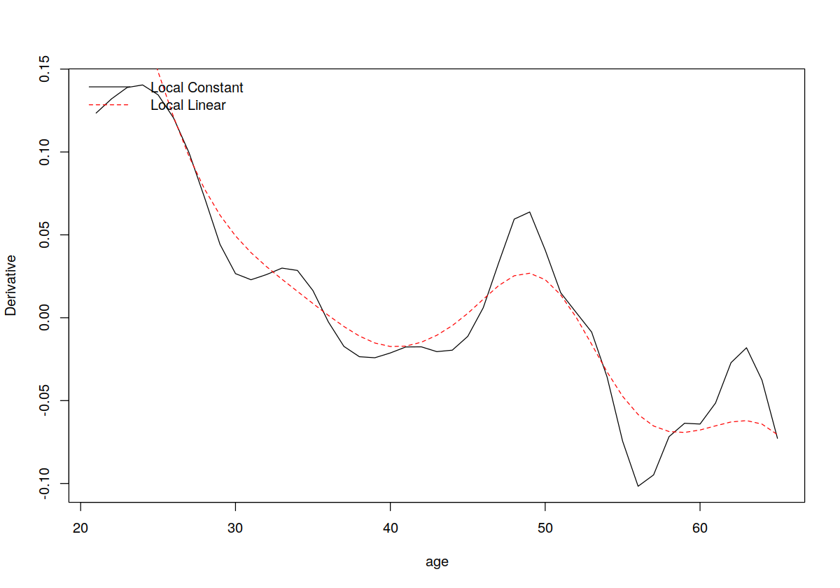
Derivatives
In [61]:
attach(cps71)

## Fit a (default) local constant model and compute the derivatives
## (since we do not explicitly call npregbw() which conducts
## least-squares cross-validated bandwidth selection by default it is
## automatically invoked when we call npreg())

model.lc <- npreg(logwage~age,gradients=TRUE)

## Plot the estimated derivatives (the colors and linetypes allow us
## to distinguish different plots on the same figure). Note that the
## function `gradients' is specific to the np package and works only
## when the argument `gradients=TRUE' is invoked when calling npreg()

plot(age,gradients(model.lc),
     ylab="Derivative",
     col=1,
     lty=1,
     type="l")

## Fit a local linear model (we use the arguments regtype="ll" to do
## this)

model.ll <- npreg(logwage~age,regtype="ll",gradients=TRUE)

## Plot the fitted values with a different color and linetype

lines(age,gradients(model.ll),col=2,lty=2)

## Add a legend

legend("topleft",
       c("Local Constant","Local Linear"),
       lty=c(1,2),
       col=c(1,2),
       bty="n")
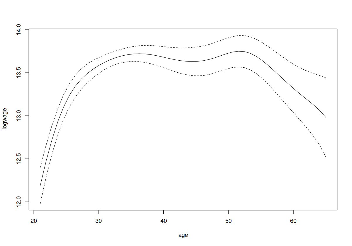
Plotting with CI
In [64]:
## Fit a local linear model (since we do not explicitly call npregbw()
## which conducts least-squares cross-validated bandwidth selection by
## default it is automatically invoked when we call npreg())
model.ll <- npreg(logwage~age,regtype="ll")
## model.ll will be an object of class `npreg'. The generic R function
## `plot' will call `npplot' when it is deployed on an object of this
## type (see ?npplot for details on supported npplot
## arguments). Calling plot on a npreg object allows you to do some
## tedious things without having to write code such as including
## confidence intervals as the following example demonstrates. Note
## also that we do not explicitly have to specify `gradients=TRUE' in
## the call to npreg() as plot (npplot) will take care of this for
## us. Below we use the asymptotic standard error estimates and then
## take +- 1.96 standard error)
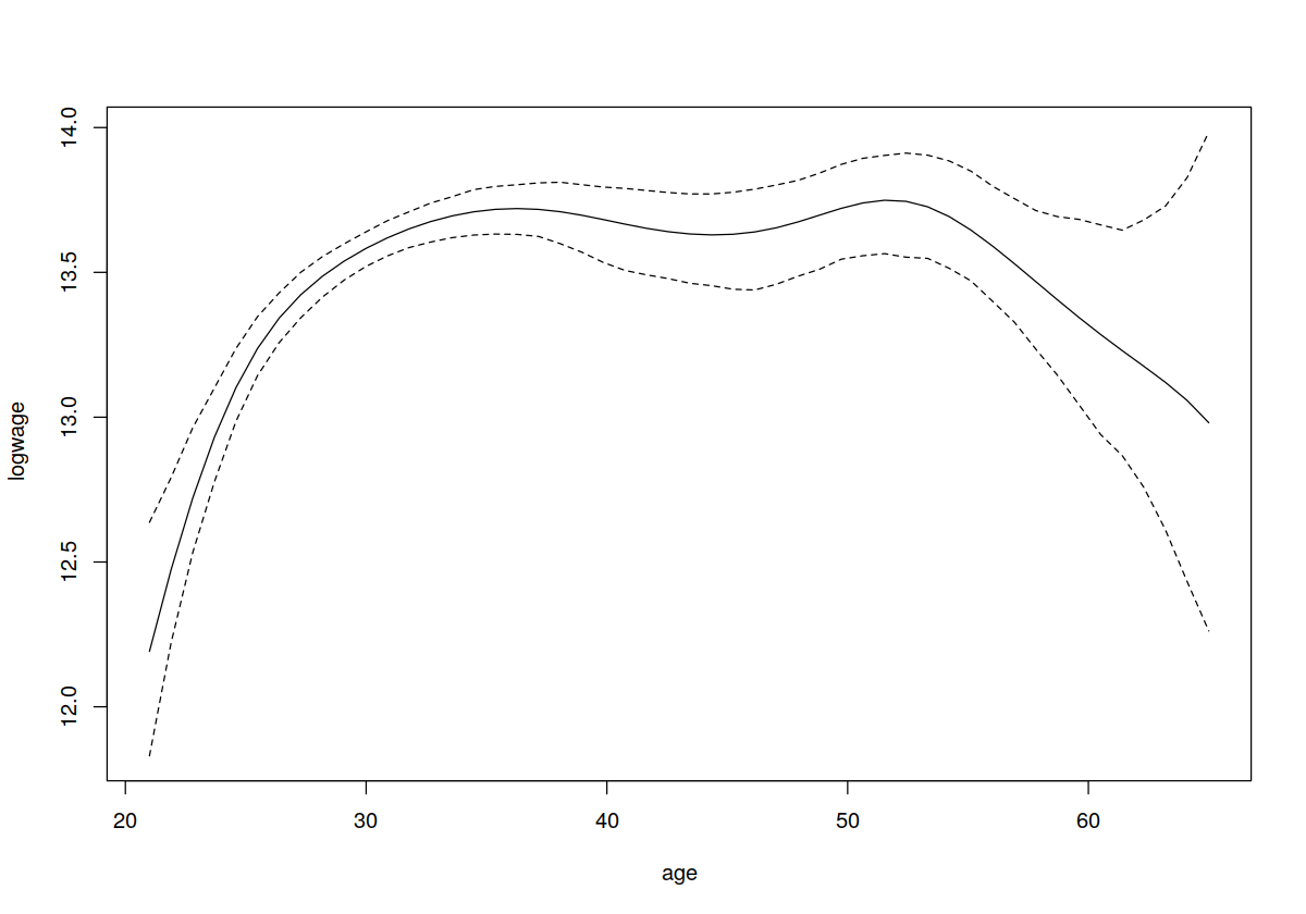
plot(model.ll,plot.errors.method="asymptotic",plot.errors.style="band")
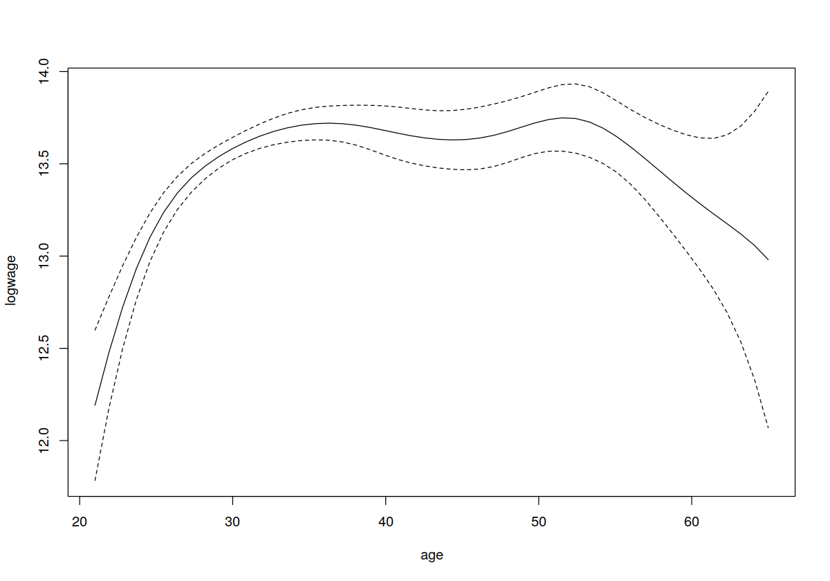
In [65]:
## We might also wish to use bootstrapping instead (here we bootstrap
## the standard errors and then take +- 1.96 standard error)

plot(model.ll,plot.errors.method="bootstrap",plot.errors.style="band")

In [66]:
## Alternately, we might compute true nonparametric confidence
## intervals using (by default) the 0.025 and 0.975 percentiles of the
## pointwise bootstrap distributions

plot(model.ll,plot.errors.method="bootstrap",plot.errors.type="quantiles",plot.errors.style="band")

In [67]:
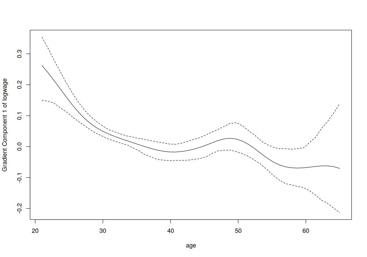
## Note that adding the argument `gradients=TRUE' to the plot call
## will automatically plot the derivatives instead

plot(model.ll,plot.errors.method="bootstrap",plot.errors.type="quantiles",plot.errors.style="band",gradients=TRUE)

Multivariate Kernel Regression
In [68]:
## Fit a local linear model (since we do not explicitly call npregbw()
## which conducts least-squares cross-validated bandwidth selection by
## default it is automatically invoked when we call npreg())

model.ll <- npreg(logwage~age,regtype="ll")

## model.ll will be an object of class `npreg'. The generic R function
## `plot' will call `npplot' when it is deployed on an object of this
## type (see ?npplot for details on supported npplot
## arguments). Calling plot on a npreg object allows you to do some
## tedious things without having to write code such as including
## confidence intervals as the following example demonstrates. Note
## also that we do not explicitly have to specify `gradients=TRUE' in
## the call to npreg() as plot (npplot) will take care of this for
## us. Below we use the asymptotic standard error estimates and then
## take +- 1.96 standard error)

plot(model.ll,plot.errors.method="asymptotic",plot.errors.style="band")

## We might also wish to use bootstrapping instead (here we bootstrap
## the standard errors and then take +- 1.96 standard error)

plot(model.ll,plot.errors.method="bootstrap",plot.errors.style="band")

## Alternately, we might compute true nonparametric confidence
## intervals using (by default) the 0.025 and 0.975 percentiles of the
## pointwise bootstrap distributions

plot(model.ll,plot.errors.method="bootstrap",plot.errors.type="quantiles",plot.errors.style="band")

## Note that adding the argument `gradients=TRUE' to the plot call
## will automatically plot the derivatives instead

plot(model.ll,plot.errors.method="bootstrap",plot.errors.type="quantiles",plot.errors.style="band",gradients=TRUE)

Comparison between Local Constant, Local Linear, and Infinite-order Locpoly
In [69]:
set.seed(42)
## Set the number of optimization restarts from different random
## initial values
nmulti <- 1
## Set the degree of the DGP (orthogonal polynomial)
degree <- 4
## Set the degree of the (overspecified) polynomial
large.poly.order <- 15
## Simulate data
n <- 500
x <- sort(runif(n,-2,2))
dgp <- function(x) {dgp<-rowSums(poly(x,degree));dgp/sd(dgp)}
y <- dgp(x) + rnorm(n,sd=.5)
In [70]:
## Load the crs package
require(crs)
## Estimate the model cross-validating both the degree and bandwidth
## (default)
model <- npglpreg(y~x,nmulti=nmulti,degree.max=10)
## Fix the order of the polynomial then cross-validate the bandwidth
## (common values are 0 for the `local constant', 1 for the `local
## linear', and try a large fixed value for comparison purposes
model.lc <- npglpreg(y~x,cv="bandwidth",degree=0,nmulti=nmulti)
model.ll <- npglpreg(y~x,cv="bandwidth",degree=1,nmulti=nmulti)
model.poly <- npglpreg(y~x,cv="bandwidth",degree=large.poly.order,nmulti=nmulti)
In [71]:
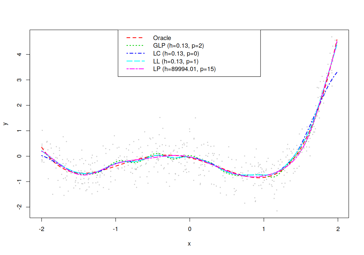
## Plot the results (DGP, Oracle LS fit, Nonparametric fit, local
## constant, local linear etc.)
## Plot the data
plot(x,y,cex=.25,col="grey")
lines(x,lm.fit<-fitted(lm(y~poly(x,degree))),col=2,lty=2,lwd=2)
lines(x,glp.fit<-fitted(model),col=3,lty=3,lwd=2)
lines(x,fitted(model.lc),col=4,lty=4,lwd=2)
lines(x,fitted(model.ll),col=5,lty=5,lwd=2)
lines(x,fitted(model.poly),col=6,lty=6,lwd=2)
legend("top",
       c("Oracle",
         paste("GLP (h=",formatC(model$bws,format="f",digits=2),", p=",model$degree,")",sep=""),
         paste("LC (h=",formatC(model.lc$bws,format="f",digits=2),", p=",model.lc$degree,")",sep=""),
         paste("LL (h=",formatC(model.ll$bws,format="f",digits=2),", p=",model.ll$degree,")",sep=""),
         paste("LP (h=",formatC(model.poly$bws,format="f",digits=2),", p=",model.poly$degree,")",sep="")),
       col=2:6,
       lty=2:6,
       lwd=rep(2,5))
In [72]:
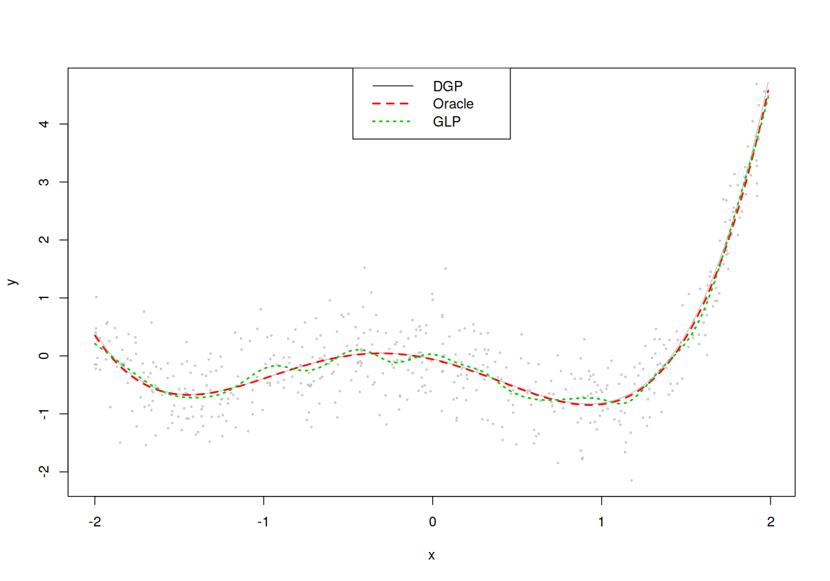
## Plot results (Oracle LS fit, Nonparametric fit only)
plot(x,y,cex=.25,col="grey")
lines(x,dgp(x),col="grey",lty=1,lwd=1)
lines(x,lm.fit<-fitted(lm(y~poly(x,degree))),col=2,lty=2,lwd=2)
lines(x,glp.fit<-fitted(model),col=3,lty=3,lwd=2)
legend("top",c("DGP","Oracle","GLP"),col=1:3,lty=1:3,lwd=c(1,2,2))
In [73]:
cbind(lm.fit,glp.fit)[seq(1,n,by=100),]
summary(model)
Nonparametric local-linear with cross-validated bandwidth selection
In [20]:
# parametric model
model.par <- lm(logwage ~ age + I(age^2), data = cps71)
summary(model.par)
In [21]:
model.np = npreg(logwage ~ age, regtype = "ll", bwmethod = "cv.aic", gradients = T, data = cps71)
summary(model.np)
In [22]:
sigtest <- npsigtest(model.np)
In [23]:
print(sigtest)
In [24]:
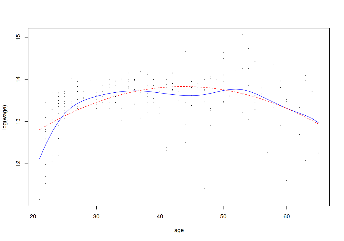
plot(cps71$age, cps71$logwage, xlab = "age", ylab = "log(wage)", cex=.1)
lines(cps71$age, fitted(model.np), lty = 1, col = "blue")
lines(cps71$age, fitted(model.par), lty = 2, col = " red")
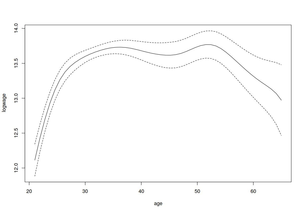
In [25]:
plot(model.np, plot.errors.method = "asymptotic")
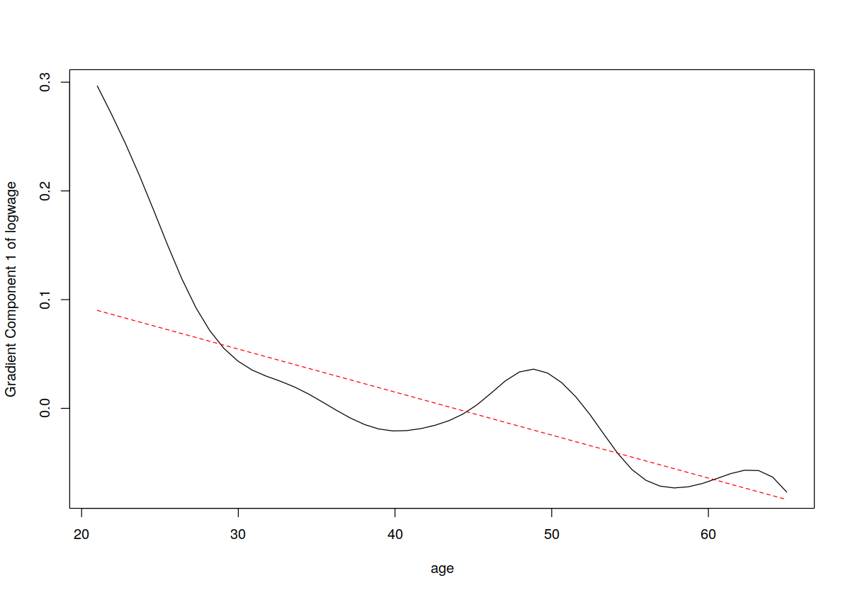
plot(model.np, gradients = TRUE)
lines(cps71$age, coef(model.par)[2]+2*cps71$age*coef(model.par)[3], lty = 2, col = "red")
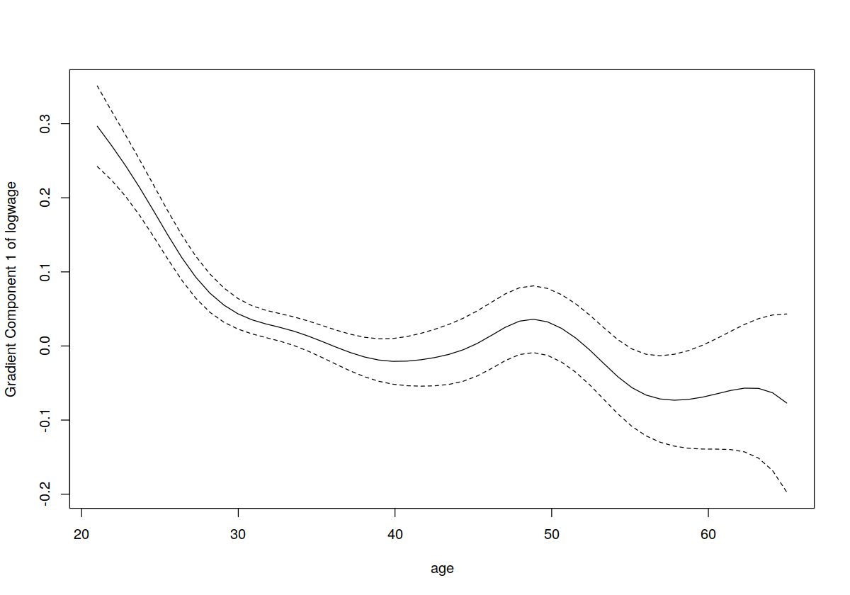
plot(model.np, gradients = TRUE, plot.errors.method = "asymptotic")
Multivariate Kernel Regression with Categorical Predictors
In [26]:
data(wage1)
wage1 %>% glimpse
In [27]:
mod.ols = lm(lwage ~ female + married + educ + exper + tenure, wage1)
summary(mod.ols)
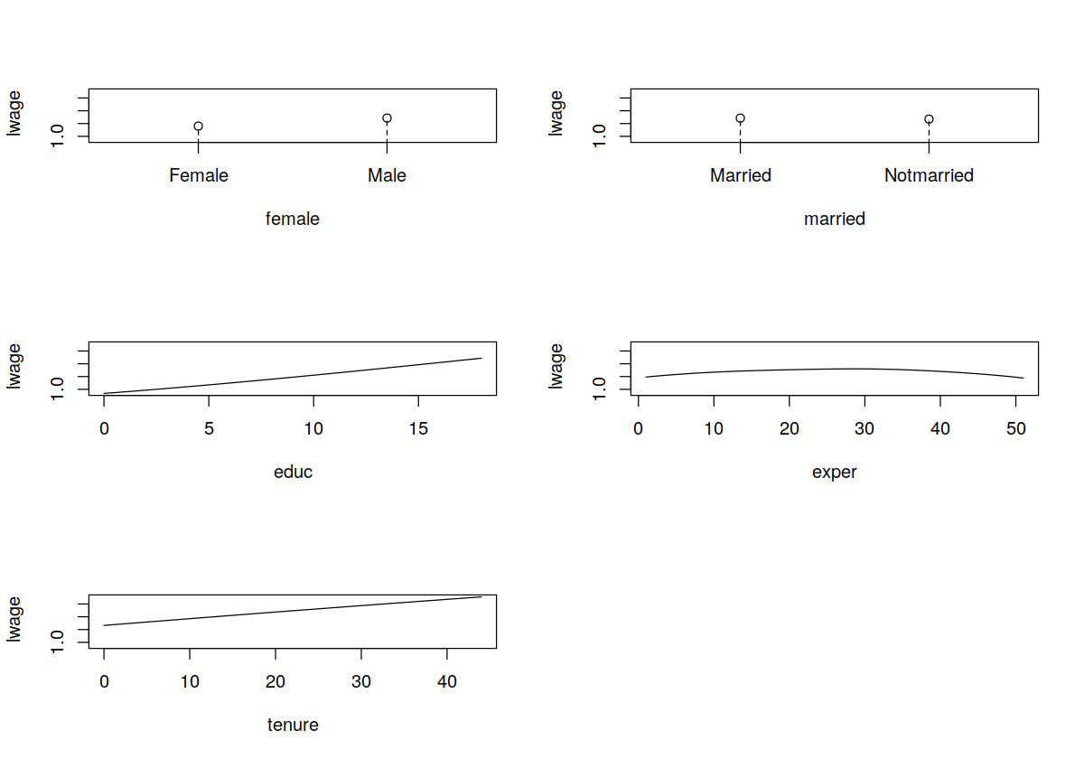
In [28]:
bw.all <- npregbw(formula = lwage ~ female + married + educ + exper + tenure,
    regtype = "ll", bwmethod = "cv.aic", data = wage1)
model.np <- npreg(bws = bw.all)
summary(model.np)
In [29]:
plot(model.np)
MSE comparison
In [34]:
set.seed(123)
ii <- sample(seq(1, nrow(wage1)), replace=FALSE)
wage1.train <- wage1[ii[1:400],]
wage1.eval <- wage1[ii[401:nrow(wage1)],]
model.ols <- lm(lwage ~ female + married + educ + exper + tenure, data = wage1.train)
fit.ols <- predict(model.ols, data = wage1.train, newdata = wage1.eval)
pse.ols <- mean((wage1.eval$lwage - fit.ols)^2)
In [35]:
bw.subset <- npregbw(formula = lwage ~ female + married + educ + exper + tenure,
 regtype = "ll", bwmethod = "cv.aic", data = wage1.train)

model.np <- npreg(bws = bw.subset)
fit.np <- predict(model.np, data = wage1.train, newdata = wage1.eval)
pse.np <- mean((wage1.eval$lwage - fit.np)^2)
In [36]:
bw.freq <- bw.subset
bw.freq$bw[1] <- 0; bw.freq$bw[2] <- 0
model.np.freq <- npreg(bws = bw.freq)
fit.np.freq <- predict(model.np.freq, data = wage1.train, newdata = wage1.eval)
pse.np.freq <- mean((wage1.eval$lwage - fit.np.freq)^2)
In [37]:
c(pse.ols, pse.np, pse.np.freq)
Discrete Outcomes
In [31]:
data("birthwt", package = "MASS")
birthwt = setDT(birthwt)
birthwt %>% glimpse
In [32]:
birthwt[, `:=`(
    low = factor(low),
    smoke = factor(smoke),
    race = factor(race),
    ht = factor(ht),
    ui = factor(ui),
    ftv = factor(ftv)
    ) ]
In [33]:
model.logit = glm(low ~ smoke + race +ht + ui + ftv + age + lwt, family = binomial(), data = birthwt)
summary(model.logit)
In [38]:
model.np <- npconmode(low ~ smoke + race + ht + ui + ftv + age + lwt,
  tol = 0.1, ftol = 0.1, data = birthwt)
Confusion Matrices
In [39]:
cm <- table(birthwt$low, ifelse(fitted(model.logit) > 0.5, 1, 0))
cm
summary(model.np)
Unconditional and Conditional CDF / PDF Estimation
Unconditional PDF/CDF
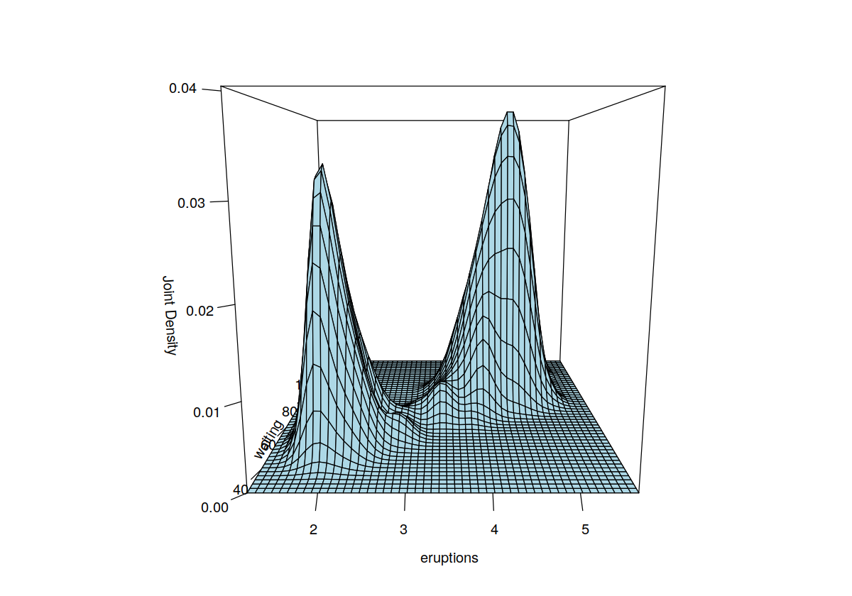
In [40]:
data("faithful", package = "datasets")
f.faithful <- npudens(~ eruptions + waiting, data = faithful)
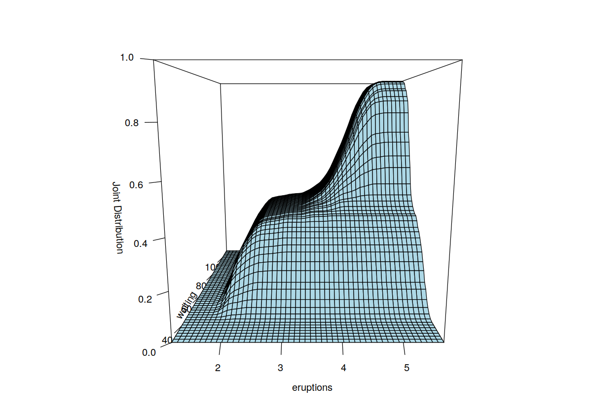
F.faithful <- npudist(~ eruptions + waiting, data = faithful)
summary(f.faithful)
In [41]:
summary(F.faithful)
In [42]:
plot(f.faithful, xtrim = -0.2, view = "fixed", main = "")
plot(F.faithful, xtrim = -0.2, view = "fixed", main = "")
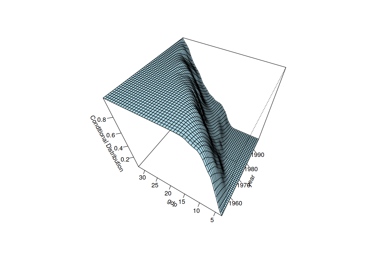
Conditional PDF / CDF
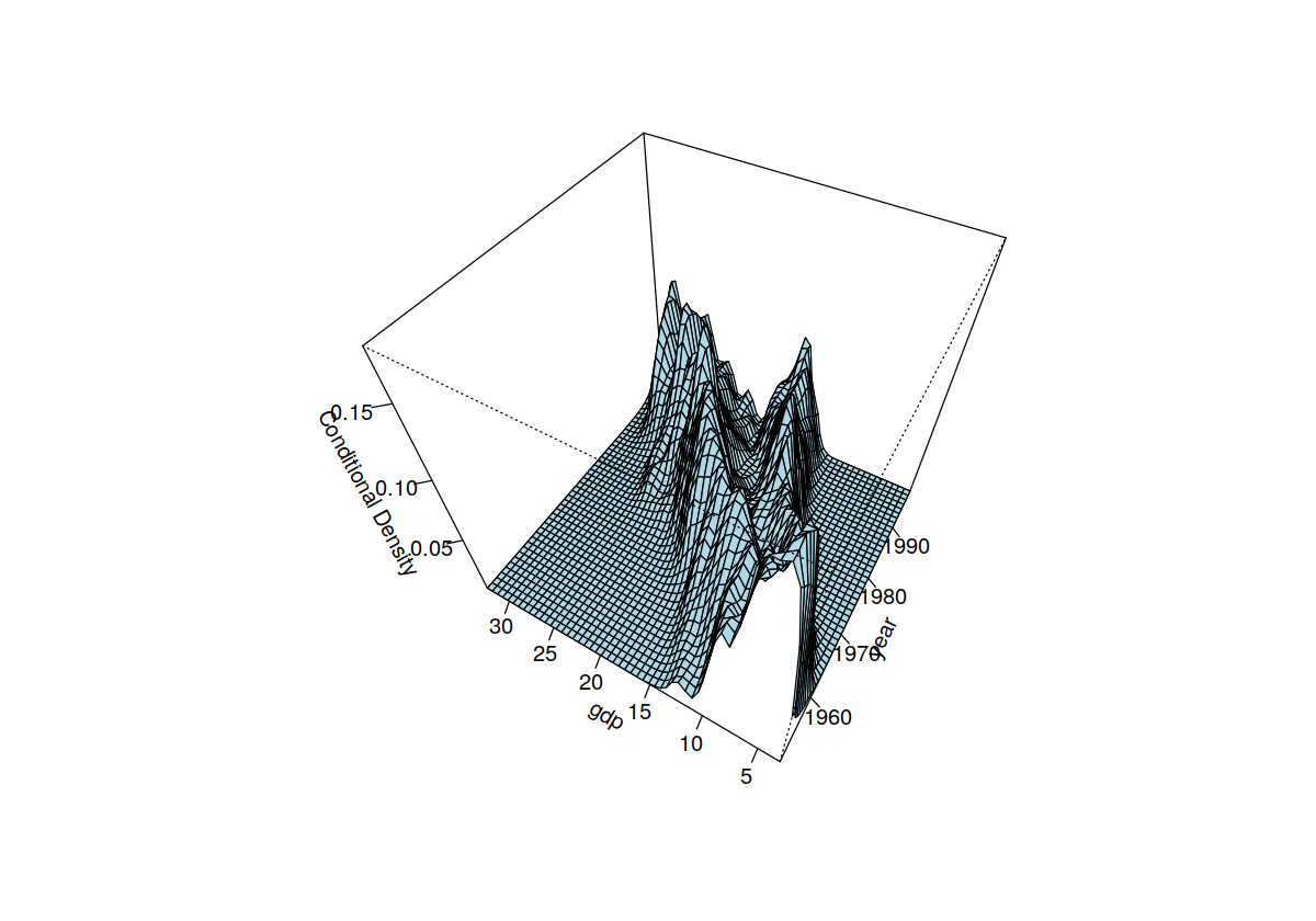
In [48]:
data("Italy")
Italy %>% glimpse
In [43]:
fhat <- npcdens(gdp ~ year, tol = 0.1, ftol = 0.1, data = Italy)
summary(fhat)
In [44]:
Fhat = npcdist(gdp ~ year, tol = 0.1, ftol = 0.1, data = Italy)
summary(Fhat)
In [45]:
plot(fhat, view = "fixed", main = "", theta = 300, phi = 50)
plot(Fhat, view = "fixed", main = "", theta = 300, phi = 50)
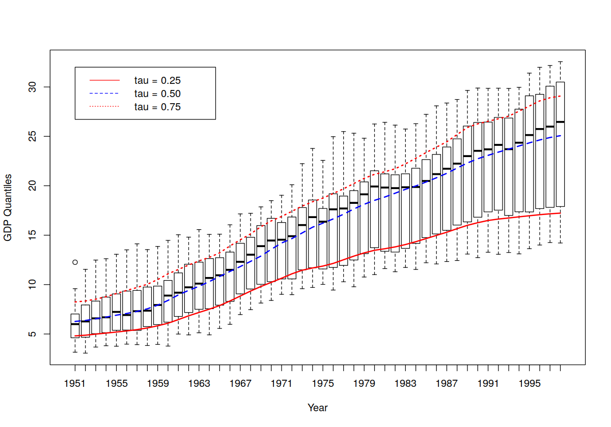
Nonparametic Quantile Regression
In [46]:
bw <- npcdistbw(formula = gdp ~ year, tol = 0.1, ftol = 0.1,
  data = Italy)
model.q0.25 <- npqreg(bws = bw, tau = 0.25)
model.q0.50 <- npqreg(bws = bw, tau = 0.50)
model.q0.75 <- npqreg(bws = bw, tau = 0.75)
In [47]:
plot(Italy$year, Italy$gdp, main = "", xlab = "Year", ylab = "GDP Quantiles")
lines(Italy$year, model.q0.25$quantile, col = "red", lty = 1, lwd = 2)
lines(Italy$year, model.q0.50$quantile, col = "blue", lty = 2, lwd = 2)
lines(Italy$year, model.q0.75$quantile, col = "red", lty = 3, lwd = 2)
legend(ordered(1951), 32, c("tau = 0.25", "tau = 0.50", "tau = 0.75"),
       lty = c(1, 2, 3), col = c("red", "blue", "red"))
Semiparametric Models
Partially Linear Model (Robinson 1988)
In [49]:
model.pl <- npplreg(lwage ~ female + married + educ + tenure | exper,
    data = wage1)
summary(model.pl)
Single Index Models
Klein and Spady
bandwidth selection via cv
In [50]:
model.index <- npindex(low ~ smoke + race + ht + ui +
  ftv + age + lwt, method = "kleinspady", gradients = TRUE,
  data = birthwt)
summary(model.index)
Ichimura
In [51]:
model.index <- npindex(lwage ~ female + married + educ + exper + tenure, data = wage1, nmulti = 1)
summary(model.index)
Semiparametric Varying-Coefficient Models
In [52]:
model.ols <- lm(lwage ~ female + married + educ + exper + tenure, data = wage1)

wage1.augmented <- wage1
wage1.augmented$dfemale <- as.integer(wage1$female == "Male")
wage1.augmented$dmarried <- as.integer(wage1$married == "Notmarried")
model.scoef <- npscoef(lwage ~ dfemale + dmarried + educ + exper + tenure | female,
                       betas = TRUE, data = wage1.augmented)
summary(model.scoef)
In [54]:
rbind(colMeans(coef(model.scoef)),
    coef(model.ols))