In [1]:
rm(list = ls())
library(LalRUtils)
libreq(data.table, magrittr, tidyverse, janitor, huxtable, knitr)
# theme_set(lal_plot_theme_d())
set.seed(42)
options(repr.plot.width = 15, repr.plot.height=12)
FECT (TWFE, Matrix Completion, IFE)
In [3]:
libreq(gsynth, devtools)
In [4]:
# devtools::install_github('xuyiqing/fastplm')
# devtools::install_github('xuyiqing/fect')
In [5]:
## for processing C++ code
libreq(Rcpp, ggplot2, GGally, grid, gridExtra)
## for parallel computing
libreq(foreach, doParallel, abind)
libreq(panelView)
In [6]:
set.seed(1234)
library(fect)
data(fect)
ls()
In [7]:
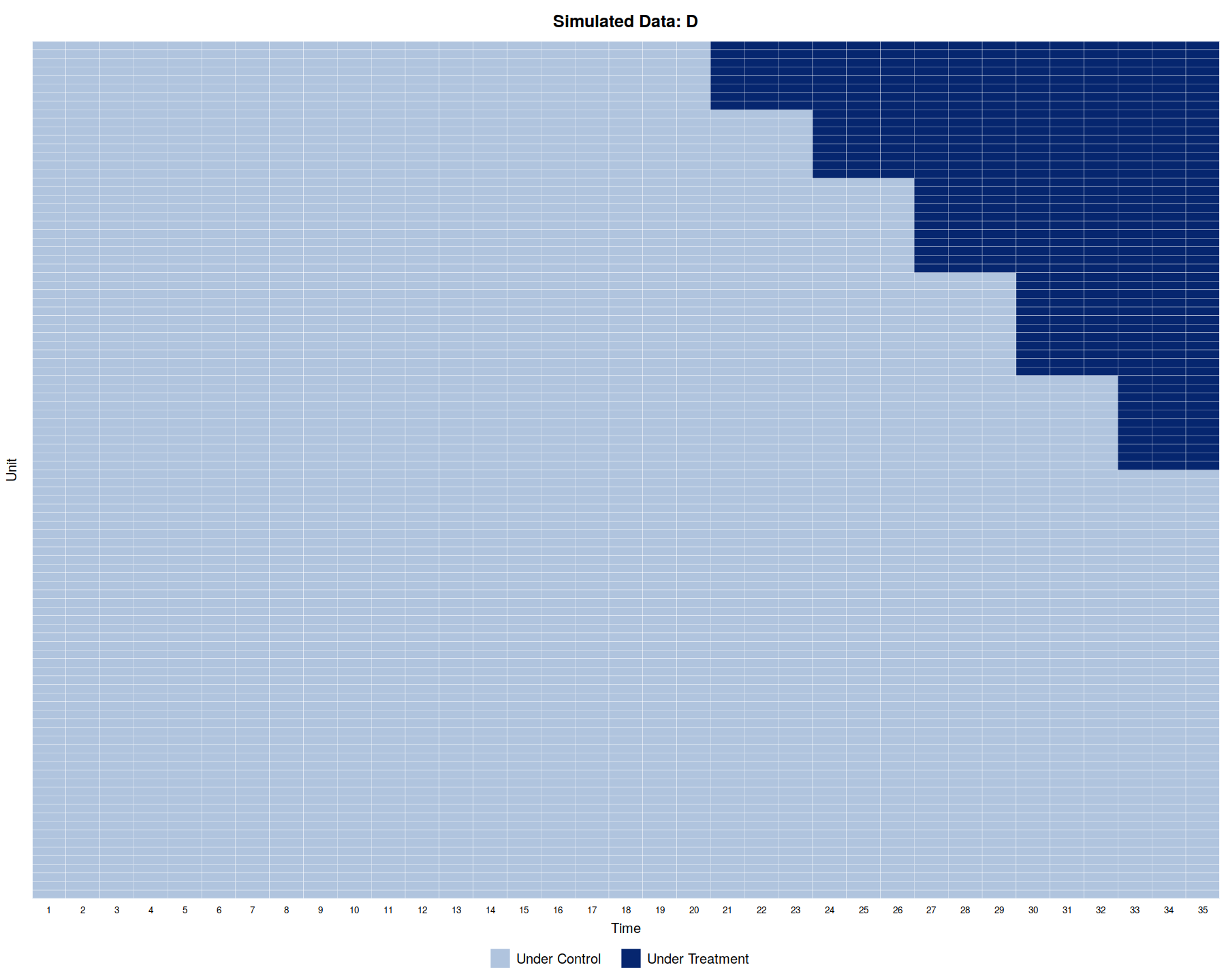
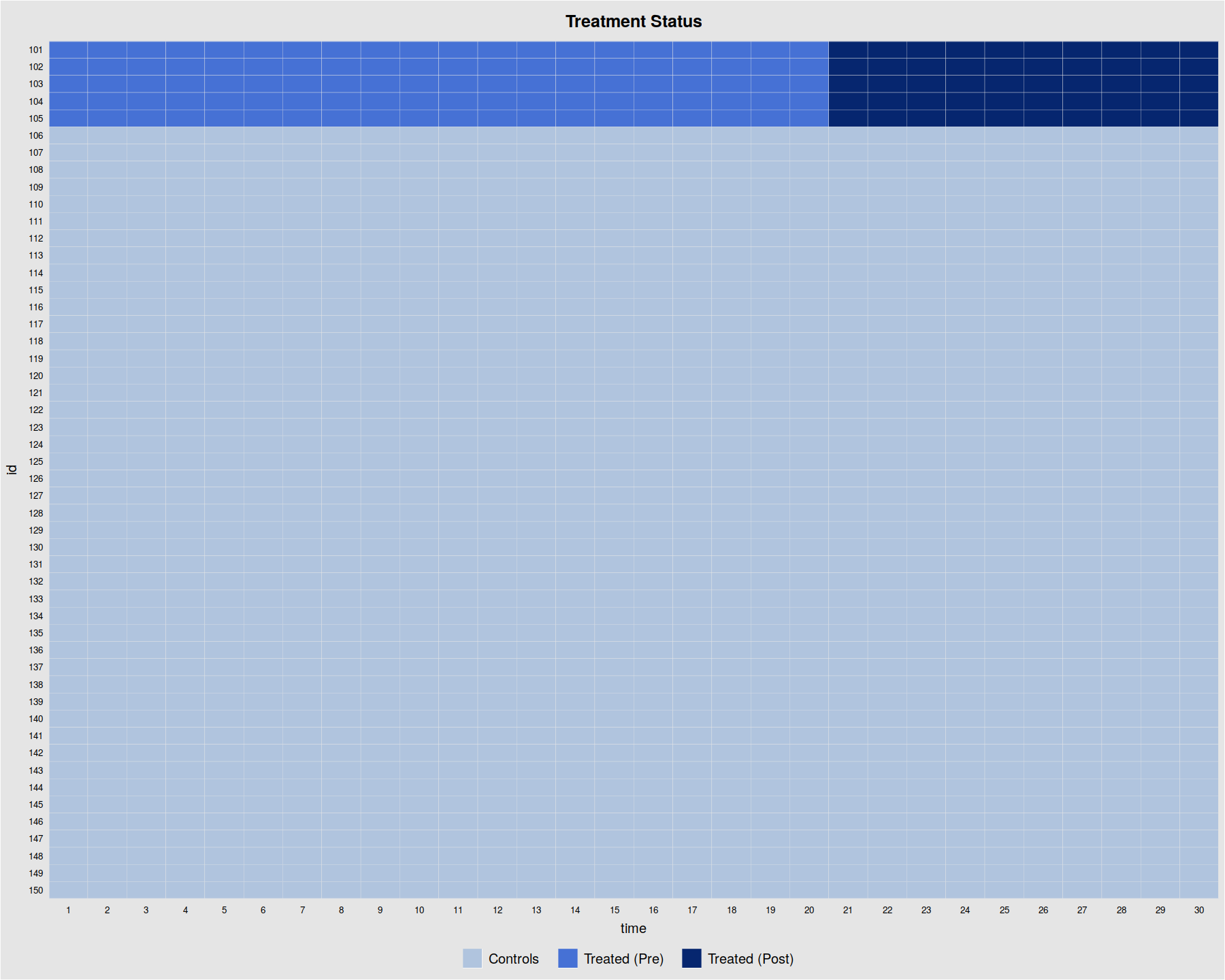
panelView(Y ~ D, data = simdata1, index = c("id","time"), by.timing = TRUE,
  axis.lab = "time", xlab = "Time", ylab = "Unit", show.id = c(1:100),
  background = "white", main = "Simulated Data: D")
In [8]:
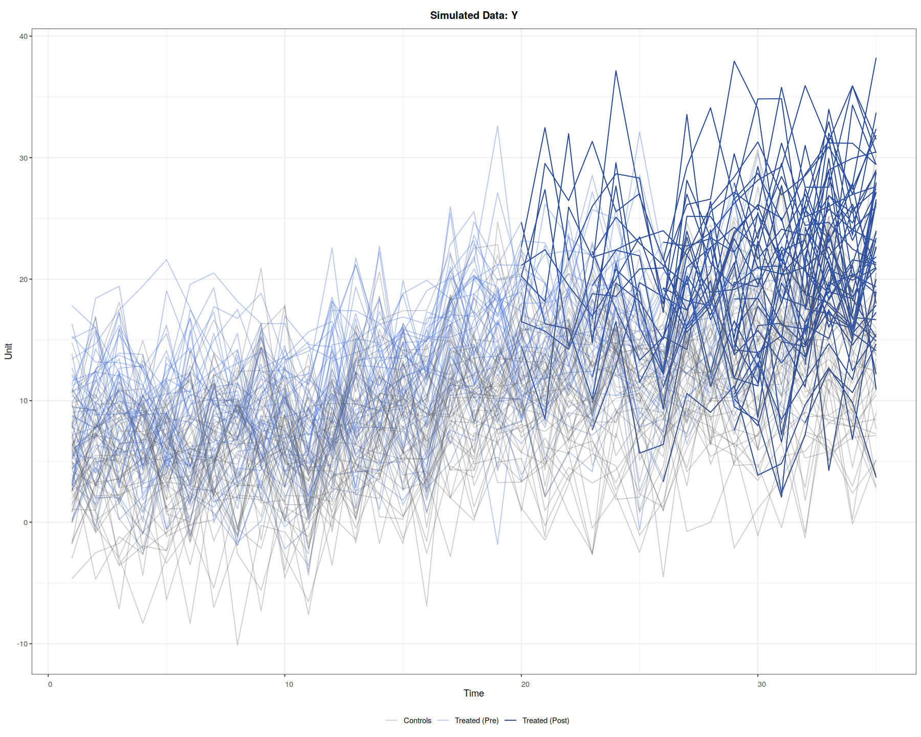
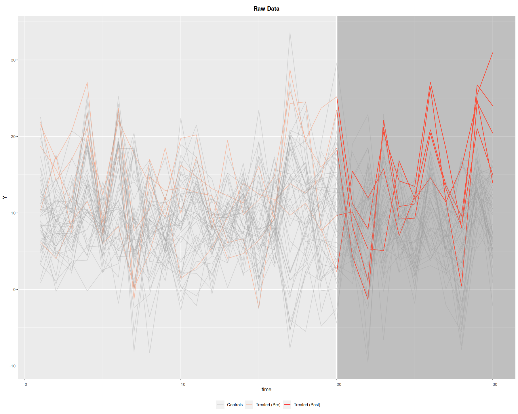
panelView(Y ~ D, data = simdata1, index = c("id","time"),
    axis.lab = "time", xlab = "Time", ylab = "Unit", show.id = c(1:100),
    theme.bw = TRUE, type = "outcome", main = "Simulated Data: Y")
In [13]:
simdata1 %>% tabyl(time, D)
TWFE
In [9]:
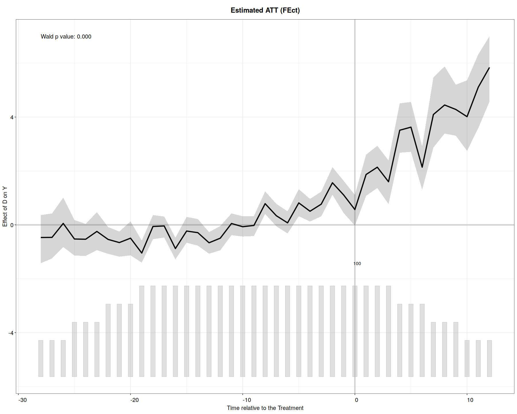
out.fe <- fect(Y ~ D + X1 + X2, data = simdata1, index = c("id","time"),
  force = "two-way", CV = TRUE, r = c(0, 5), se = TRUE, wald = TRUE,
  nboots = 200, parallel = TRUE)
In [10]:
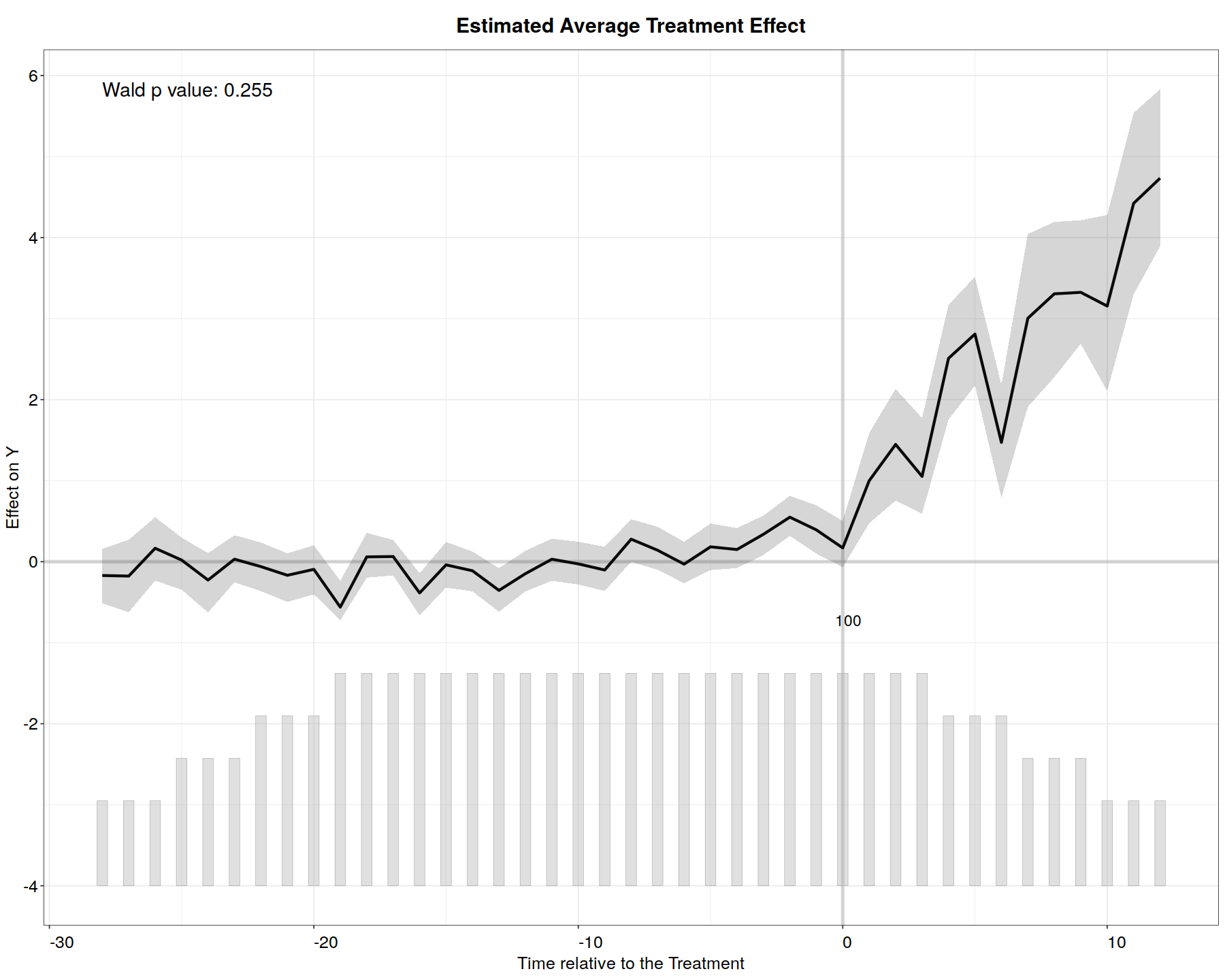
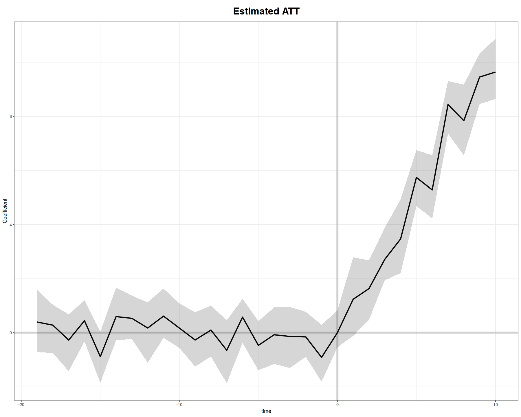
plot(out.fe, main = "Estimated ATT (FEct)", ylab = "Effect of D on Y",
  cex.main = 0.8, cex.lab = 0.8, cex.axis = 0.8, cex.text = 0.7)
Interactive Fixed Effects
In [11]:
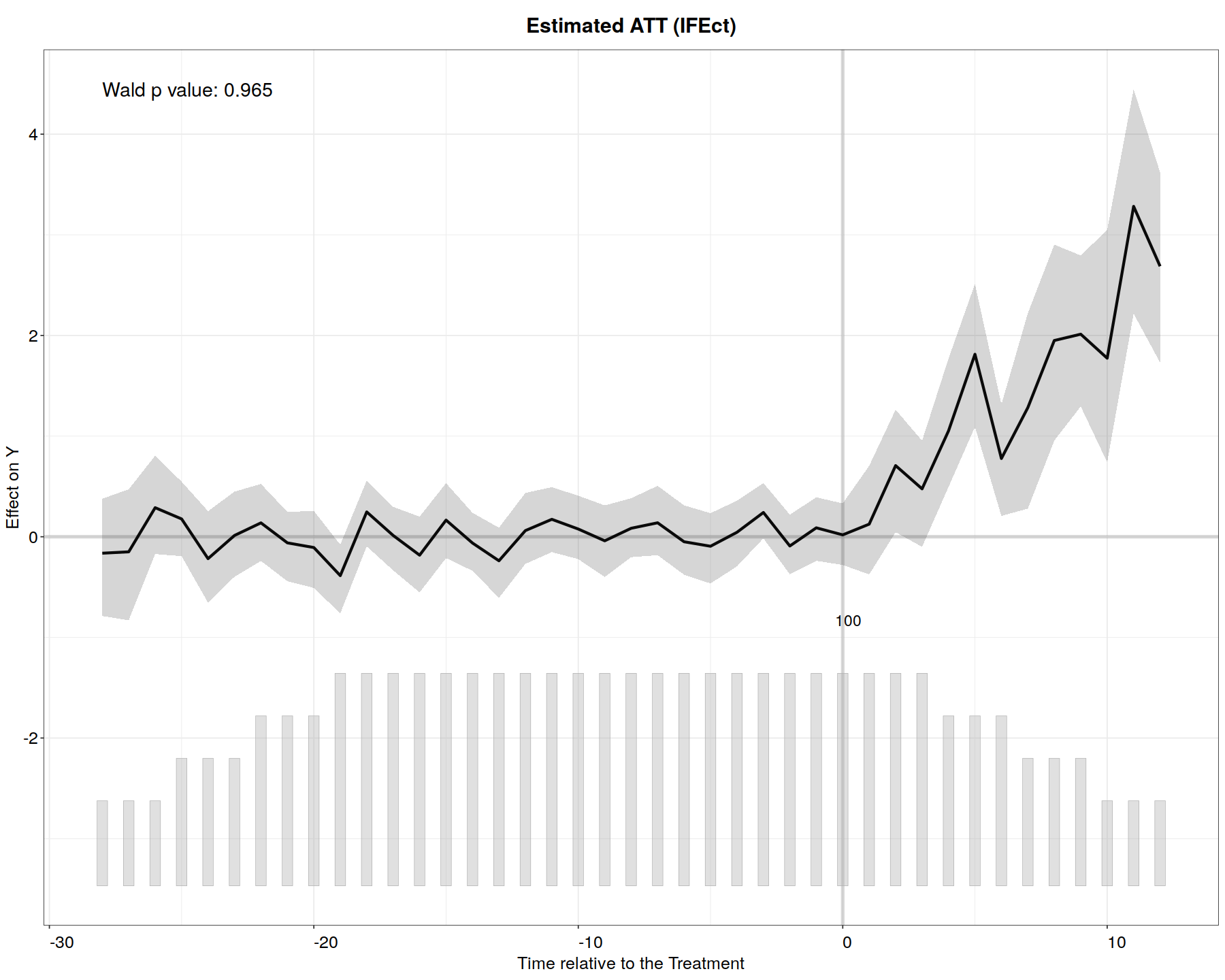
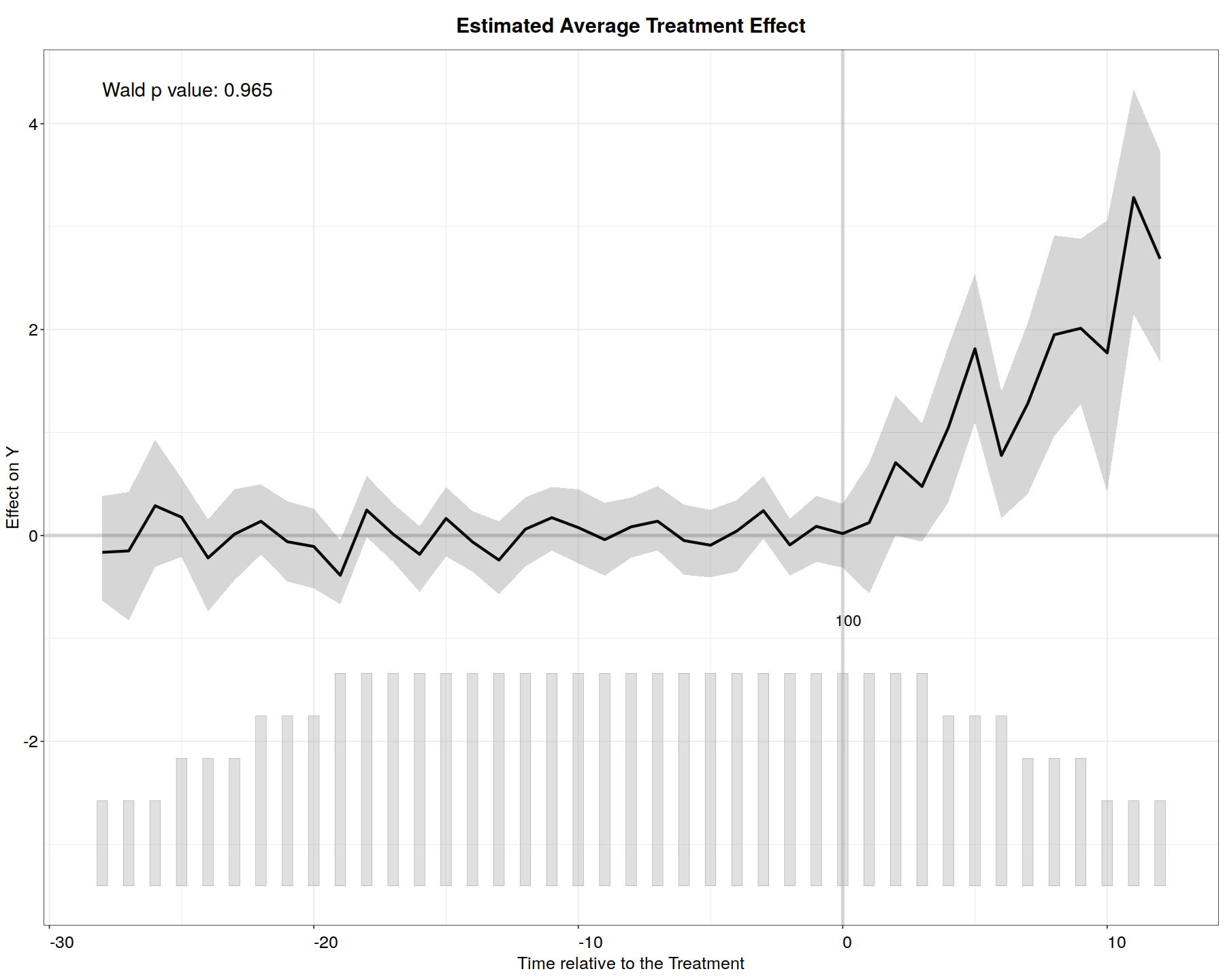
out.ife <- fect(Y ~ D + X1 + X2, data = simdata1, index = c("id","time"),
          force = "two-way", method = "ife", CV = TRUE, r = c(0, 5), wald = TRUE,
          se = TRUE, nboots = 200, parallel = TRUE)
In [14]:
plot(out.ife, main = "Estimated ATT (IFEct)")
Matrix Completion
In [15]:
out.mc <- fect(Y ~ D + X1 + X2, data = simdata1, index = c("id","time"),
          force = "two-way", method = "mc", CV = TRUE, wald = TRUE,
          se = TRUE, nboots = 200, parallel = TRUE)
In [17]:
plot(out.mc)
Both
In [16]:
out.both <- fect(Y ~ D + X1 + X2, data = simdata1, index = c("id","time"),
          force = "two-way", method = "both", CV = TRUE, wald = TRUE,
          se = TRUE, nboots = 200, parallel = TRUE)
In [18]:
plot(out.both)
Gsynth
In [19]:
data(gsynth)
ls()
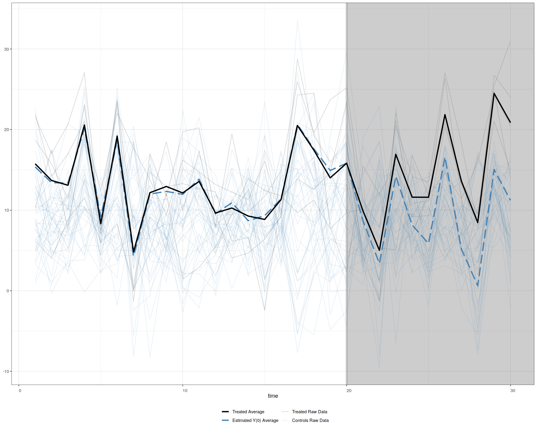
In [21]:
head(simdata)
panelView(Y ~ D, data = simdata,  index = c("id","time"), pre.post = TRUE)
panelView(Y ~ D, data = simdata,  index = c("id","time"), type = "outcome")
In [22]:
system.time(
    out <- gsynth(Y ~ D + X1 + X2, data = simdata, index = c("id","time"),
    force = "two-way", CV = TRUE, r = c(0, 5), se = TRUE,
    inference = "parametric", nboots = 200, parallel = TRUE)
)
In [27]:
plot(out, theme.bw = T) # by default
plot(out, type = "counterfactual", raw = "all", main="", theme.bw = T)
EDR Example
In [28]:
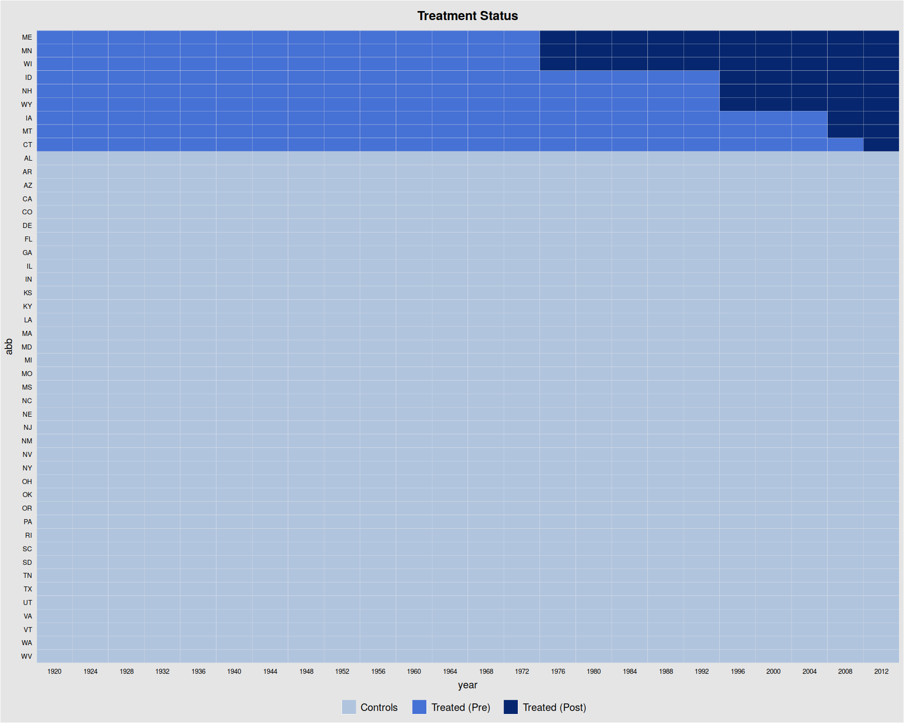
panelView(turnout ~ policy_edr, data = turnout,  index = c("abb","year"),
          pre.post = TRUE, by.timing = TRUE)
In [29]:
out0 <- gsynth(turnout ~ policy_edr + policy_mail_in + policy_motor,
               data = turnout, index = c("abb","year"), se = TRUE, inference = "parametric",
               r = 0,
               CV = FALSE, force = "two-way", nboots = 200, seed = 02139)
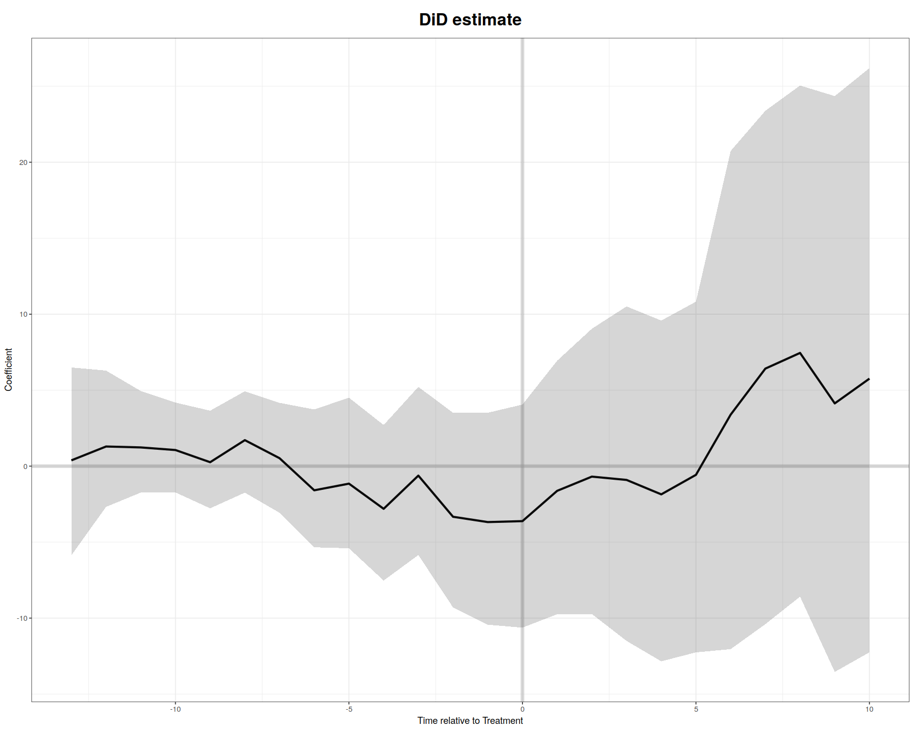
In [31]:
plot(out0, main = "DiD estimate", theme.bw = T)
In [32]:
out <- gsynth(turnout ~ policy_edr + policy_mail_in + policy_motor,
              data = turnout,  index = c("abb","year"), se = TRUE, inference = "parametric",
              r = c(0, 5), CV = TRUE, force = "two-way", nboots = 200, seed = 02139)
In [34]:
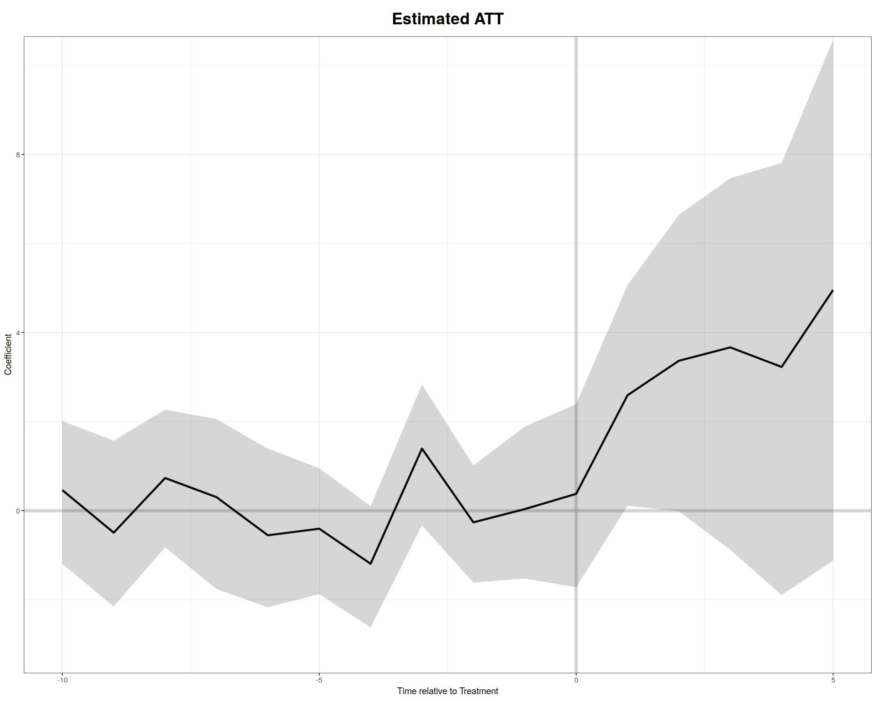
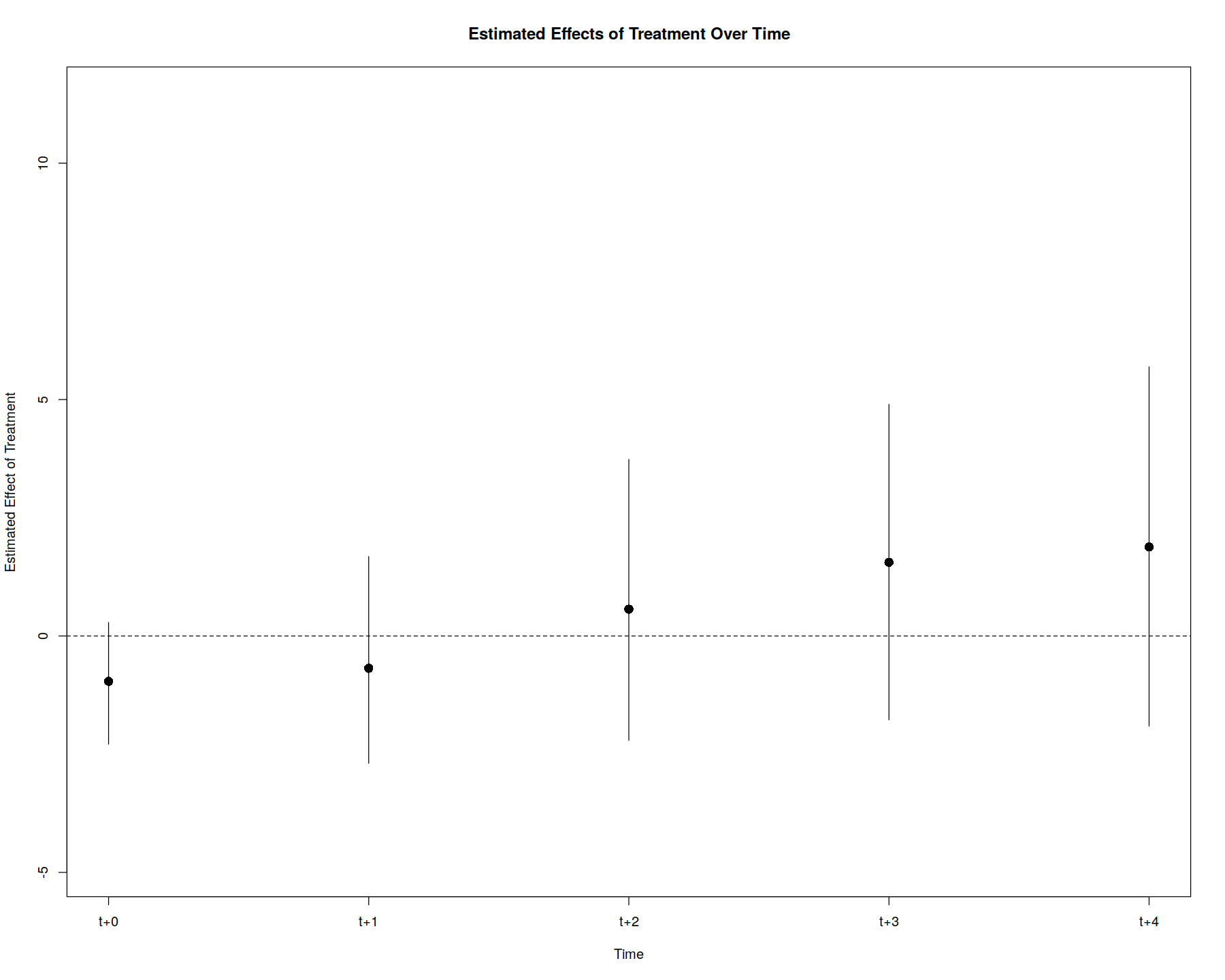
plot(out, type = "gap", xlim = c(-10, 5), ylim=c(-3,10), theme.bw = T)
In [35]:
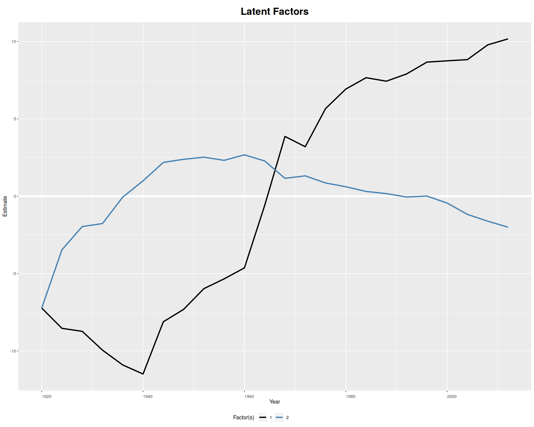
plot(out, type = "factors", xlab="Year")
Bayesian Time Series
Structural Time Series - CausalImpact
In [36]:
libreq(CausalImpact)
In [38]:
set.seed(1)
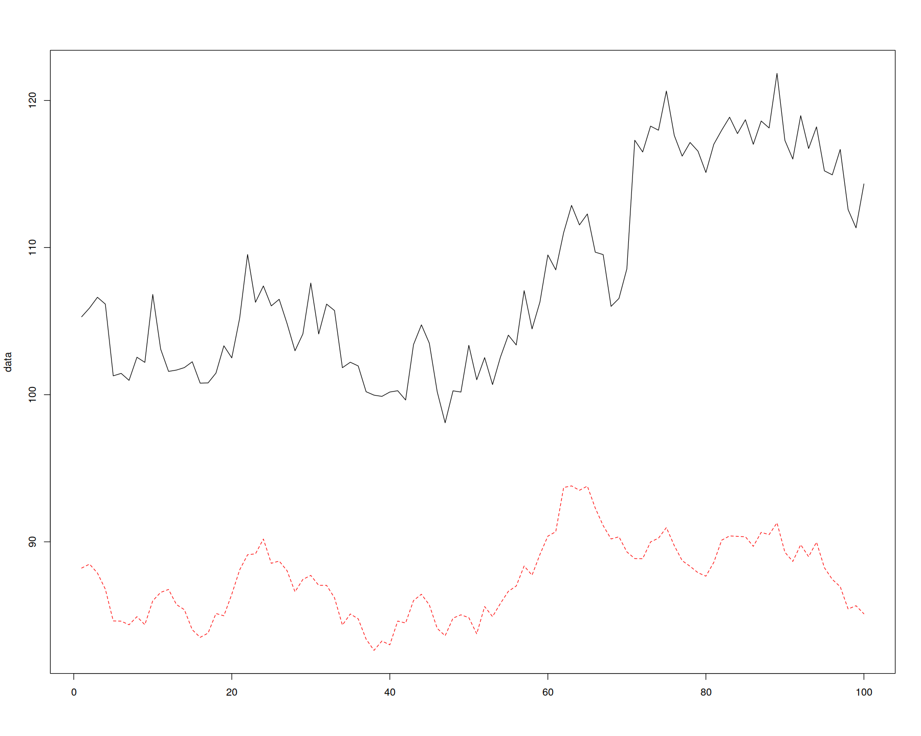
x1 <- 100 + arima.sim(model = list(ar = 0.999), n = 100)
y <- 1.2 * x1 + rnorm(100)
y[71:100] <- y[71:100] + 10
data <- cbind(y, x1)
head(data)
In [39]:
matplot(data, type = "l")
In [40]:
pre.period <- c(1, 70)
post.period <- c(71, 100)
impact <- CausalImpact(data, pre.period, post.period)
In [41]:
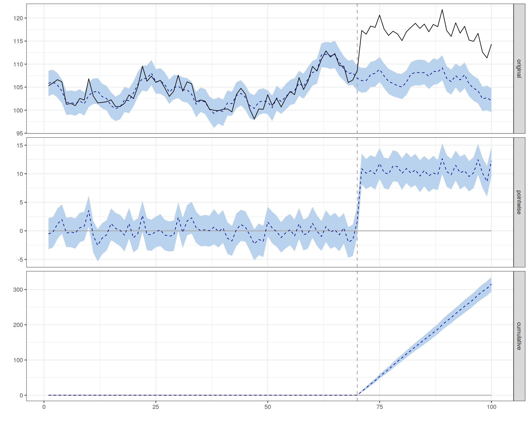
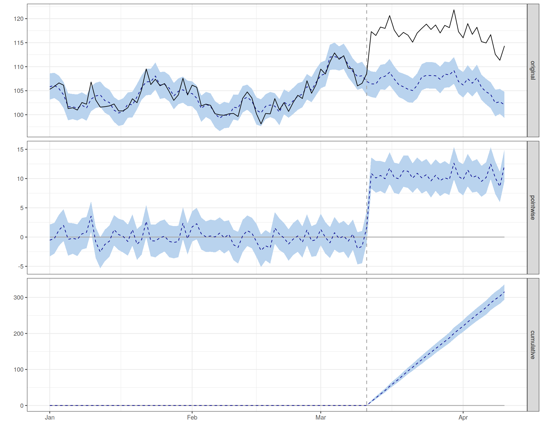
plot(impact)
In [42]:
time.points <- seq.Date(as.Date("2014-01-01"), by = 1, length.out = 100)
data <- zoo(cbind(y, x1), time.points)
pre.period <- as.Date(c("2014-01-01", "2014-03-11"))
post.period <- as.Date(c("2014-03-12", "2014-04-10"))
head(data)
In [43]:
impact <- CausalImpact(data, pre.period, post.period)
plot(impact)
PanelMatch
In [3]:
libreq(PanelMatch)
In [5]:
dem %>% head
In [4]:
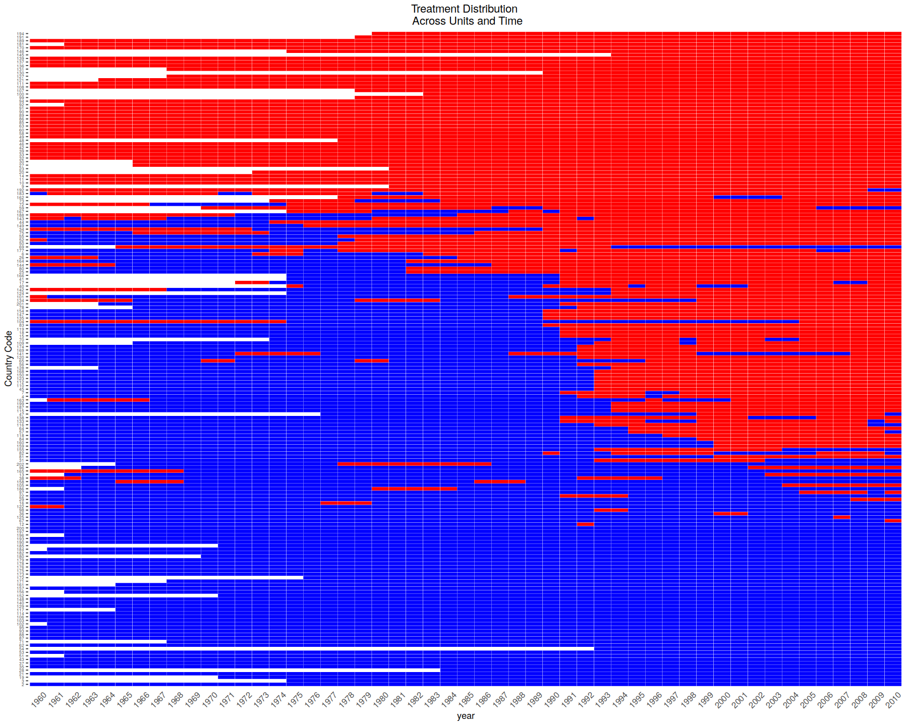
DisplayTreatment(unit.id = "wbcode2",
                 time.id = "year", legend.position = "none",
                 xlab = "year", ylab = "Country Code",
                 treatment = "dem", data = dem)
Match on pre-trends in tradewb
In [19]:
PM.results <- PanelMatch(lag = 4, time.id = "year", unit.id = "wbcode2",
                         treatment = "dem", refinement.method = "mahalanobis", # use Mahalanobis distance
                         data = dem, match.missing = TRUE,
                         covs.formula = ~ y,
                         size.match = 5, qoi = "att" , outcome.var = "y",
                         lead = 0:4, forbid.treatment.reversal = FALSE,
                         use.diagonal.variance.matrix = TRUE)
In [20]:
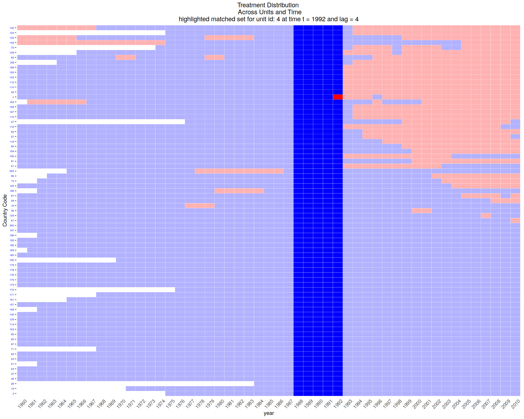
# extract the first matched set
mset <- PM.results$att[1]

DisplayTreatment(unit.id = "wbcode2",
                 time.id = "year", legend.position = "none",
                 xlab = "year", ylab = "Country Code",
                 treatment = "dem", data = dem,
                 matched.set = mset, # this way we highlight the particular set
                 show.set.only = TRUE)
In [21]:
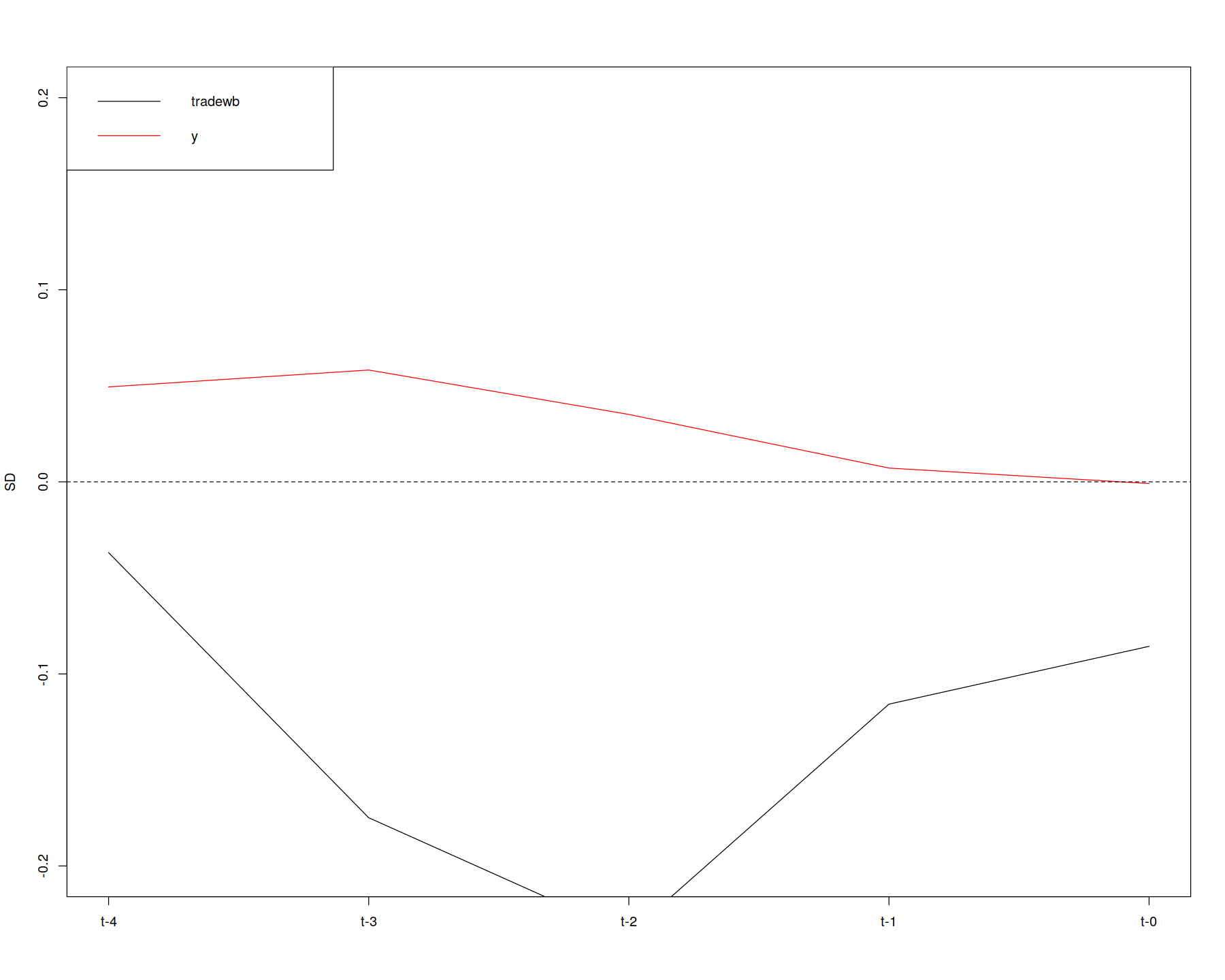
# compare with sets that have had various refinements applied

get_covariate_balance(PM.results$att,
                      data = dem,
                      covariates = c("tradewb", "y"),
                      plot = FALSE)

get_covariate_balance(PM.results$att,
                      data = dem,
                      covariates = c("tradewb", "y"),
                      plot = TRUE, # visualize by setting plot to TRUE
                      ylim = c(-.2, .2))
Estimate after matching
In [17]:
PE.results <- PanelEstimate(sets = PM.results, data = dem)

summary(PE.results)
plot(PE.results)
DiD and double-robust DiD
In [2]:
library(devtools)
In [8]:
# devtools::install_github("bcallaway11/did")
libreq(ggpubr)
In [4]:
library(did)
data(mpdta)
The dataset contains 500 observations of county-level teen employment rates from 2003-2007. Some states are first treated in 2004, some in 2006, and some in 2007 (see the paper for more details). The important variables in the dataset are
lemp This is the log of county-level teen employment. It is the outcome variable
first.treat This is the period when a state first increases its minimum wage. It can be 2004, 2006, or 2007. It is the variable that defines group in this application
year This is the year and is the time variable
countyreal This is an id number for each county and provides the individual identifier in this panel data context
In [5]:
out <- att_gt(yname="lemp",
              first.treat.name="first.treat",
              idname="countyreal",
              tname="year",
              xformla=~1,
              data=mpdta,
              estMethod="reg",
              printdetails=FALSE,
              )
In [6]:
summary(out)
In [9]:
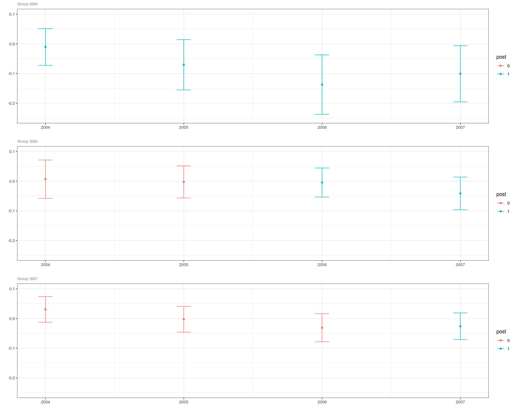
ggdid(out, ylim=c(-.25,.1))
In [10]:
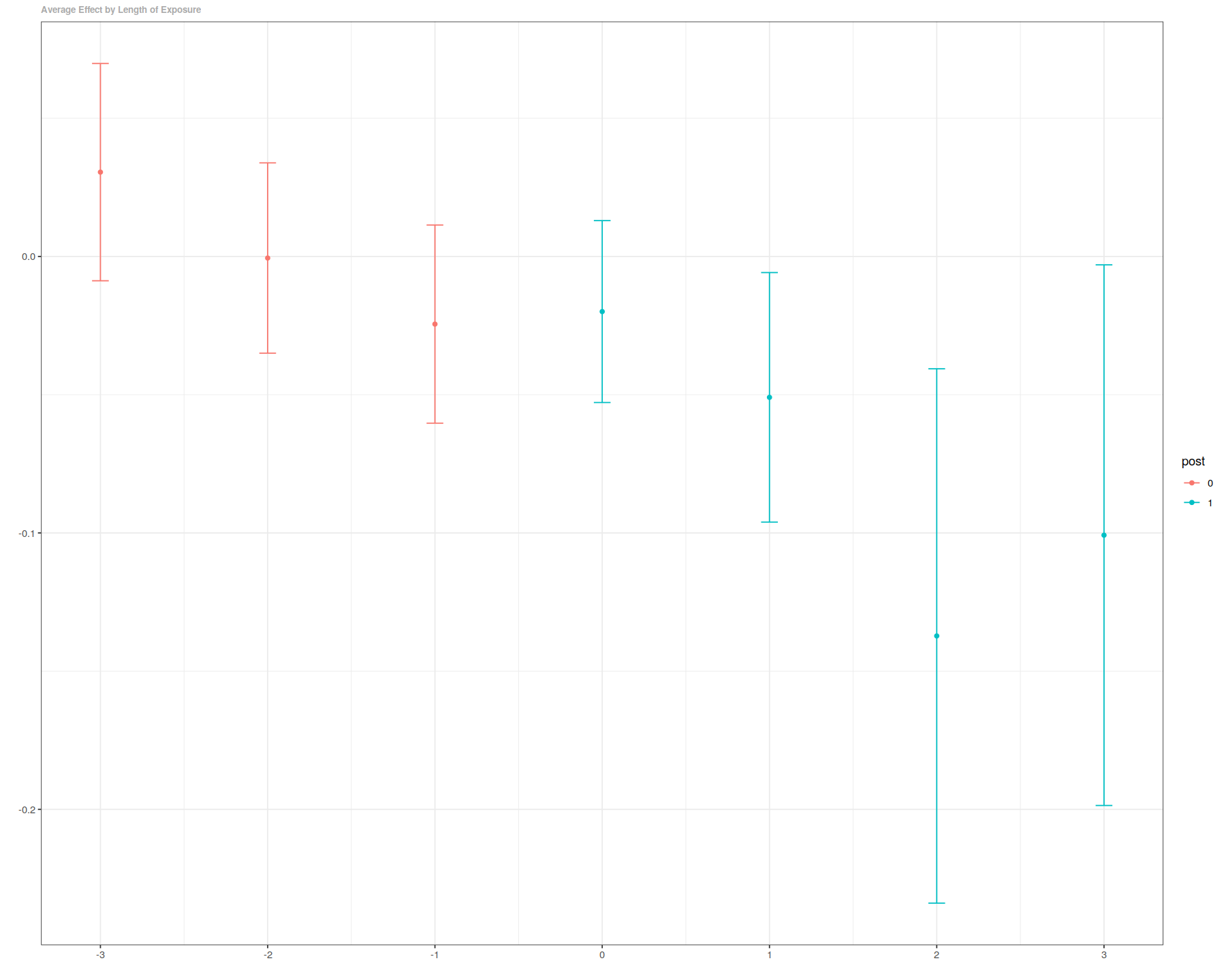
es <- aggte(out, type="dynamic")
In [12]:
summary(es)
ggdid(es)
DRDID
In [13]:
devtools::install_github("pedrohcgs/DRDID")
DrDID with inverse-probability-tilting
In [14]:
library(DRDID)
# Load data in long format that comes in the DRDID package
data(nsw_long)
# Form the Lalonde sample with CPS comparison group
eval_lalonde_cps <- subset(nsw_long, nsw_long$treated == 0 | nsw_long$sample == 2)
In [15]:
# Implement improved locally efficient DR DID:
out <- drdid(yname = "re", tname = "year", idname = "id", dname = "experimental",
             xformla= ~ age + educ + black + married + nodegree + hisp + re74,
             data = eval_lalonde_cps, panel = TRUE)
summary(out)
TWFE
In [16]:
# Form the Lalonde sample with CPS comparison group
eval_lalonde_cps <- subset(nsw, nsw$treated == 0 | nsw$sample == 2)
# Select some covariates
covX = as.matrix(cbind(eval_lalonde_cps$age, eval_lalonde_cps$educ,
                       eval_lalonde_cps$black, eval_lalonde_cps$married,
                       eval_lalonde_cps$nodegree, eval_lalonde_cps$hisp,
                       eval_lalonde_cps$re74))
# Implement TWFE DID with panel data
twfe_did_panel(y1 = eval_lalonde_cps$re78, y0 = eval_lalonde_cps$re75,
               D = eval_lalonde_cps$experimental,
               covariates = covX)
In [22]:
libreq(scul, tidyverse, glmnet, pBrackets, knitr, kableExtra, cowplot, formattable, Synth)
In [23]:
data(cigarette_sales)
## -----------------------------------------------------------------------------
dim(cigarette_sales)

head(cigarette_sales[,1:6])
In [24]:
AllYData <- cigarette_sales[, 1:2]
AllXData <- cigarette_sales %>%
  select(-c("year", "cigsale_6", "retprice_6"))
In [25]:
## -----------------------------------------------------------------------------
processed.AllYData <- Preprocess(AllYData)

TreatmentBeginsAt <- 19 # Here the 18th row is 1988
PostPeriodLength <- nrow(processed.AllYData) - TreatmentBeginsAt + 1
PrePeriodLength <- TreatmentBeginsAt-1
NumberInitialTimePeriods <- 5
processed.AllYData <- PreprocessSubset(processed.AllYData,
                                       TreatmentBeginsAt ,
                                       NumberInitialTimePeriods,
                                       PostPeriodLength,
                                       PrePeriodLength)
In [26]:
## -----------------------------------------------------------------------------
SCUL.input <- OrganizeDataAndSetup (
    time =  data.frame(AllYData[, 1]),
    y = data.frame(AllYData[, 2]),
    TreatmentBeginsAt = TreatmentBeginsAt,
    x.DonorPool = AllXData[, -1],
    CohensDThreshold = 0.25,
    NumberInitialTimePeriods = NumberInitialTimePeriods,
    TrainingPostPeriodLength = 7,
    x.PlaceboPool = AllXData[, -1],
    OutputFilePath="vignette_output/"
)
In [27]:
GraphTargetData()
In [28]:
## ---- echo = FALSE------------------------------------------------------------
first_guess_lasso = glmnet(as.matrix(SCUL.input$x.DonorPool[(1:TreatmentBeginsAt-1),]), as.matrix(SCUL.input$y[(1:TreatmentBeginsAt-1),]))
In [29]:
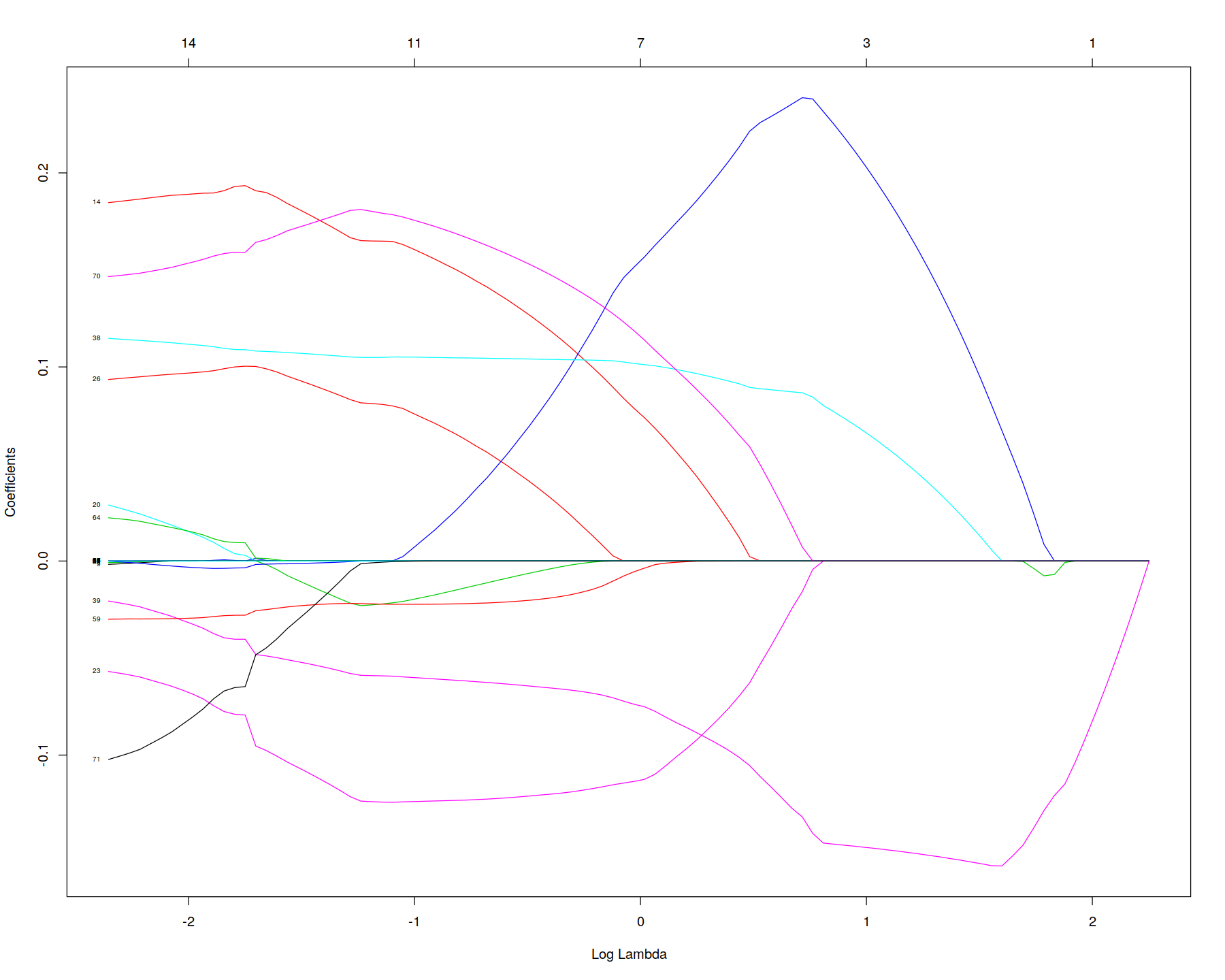
## ---- fig.height=5.33, fig.width=8, warning = FALSE, fig.align = "center", echo = FALSE, out.width = '100%'----
plot(first_guess_lasso, "lambda", label = TRUE )
In [30]:
# Create a dataframe of the treated data
data_to_plot_scul_vary_lambda <- data.frame(SCUL.input$time, SCUL.input$y)
# Label the columns
colnames(data_to_plot_scul_vary_lambda) <- c("time", "actual_y")
# Create four naive predictions that are based on random lambdas
data_to_plot_scul_vary_lambda$naive_prediction_1 <-
predict(
x = as.matrix(SCUL.input$x.DonorPool[(1:TreatmentBeginsAt-1),]),
y = as.matrix(SCUL.input$y[(1:TreatmentBeginsAt-1),]),
newx = as.matrix(SCUL.input$x.DonorPool),
first_guess_lasso,
s = first_guess_lasso$lambda[1],
exact = TRUE
)
data_to_plot_scul_vary_lambda$naive_prediction_2 <-
predict(
x = as.matrix(SCUL.input$x.DonorPool[(1:TreatmentBeginsAt-1),]),
y = as.matrix(SCUL.input$y[(1:TreatmentBeginsAt-1),]),
newx = as.matrix(SCUL.input$x.DonorPool),
first_guess_lasso,
s = first_guess_lasso$lambda[round(length(first_guess_lasso$lambda)/10)],
exact = TRUE
)
data_to_plot_scul_vary_lambda$naive_prediction_3 <-
predict(
x = as.matrix(SCUL.input$x.DonorPool[(1:TreatmentBeginsAt-1),]),
y = as.matrix(SCUL.input$y[(1:TreatmentBeginsAt-1),]),
newx = as.matrix(SCUL.input$x.DonorPool),
first_guess_lasso,
s = first_guess_lasso$lambda[round(length(first_guess_lasso$lambda)/5)],
exact = TRUE
)
data_to_plot_scul_vary_lambda$naive_prediction_4 <-
predict(
x = as.matrix(SCUL.input$x.DonorPool[(1:TreatmentBeginsAt-1),]),
y = as.matrix(SCUL.input$y[(1:TreatmentBeginsAt-1),]),
newx = as.matrix(SCUL.input$x.DonorPool),
first_guess_lasso,
s = 0,
exact = TRUE
)
# Plot these variables
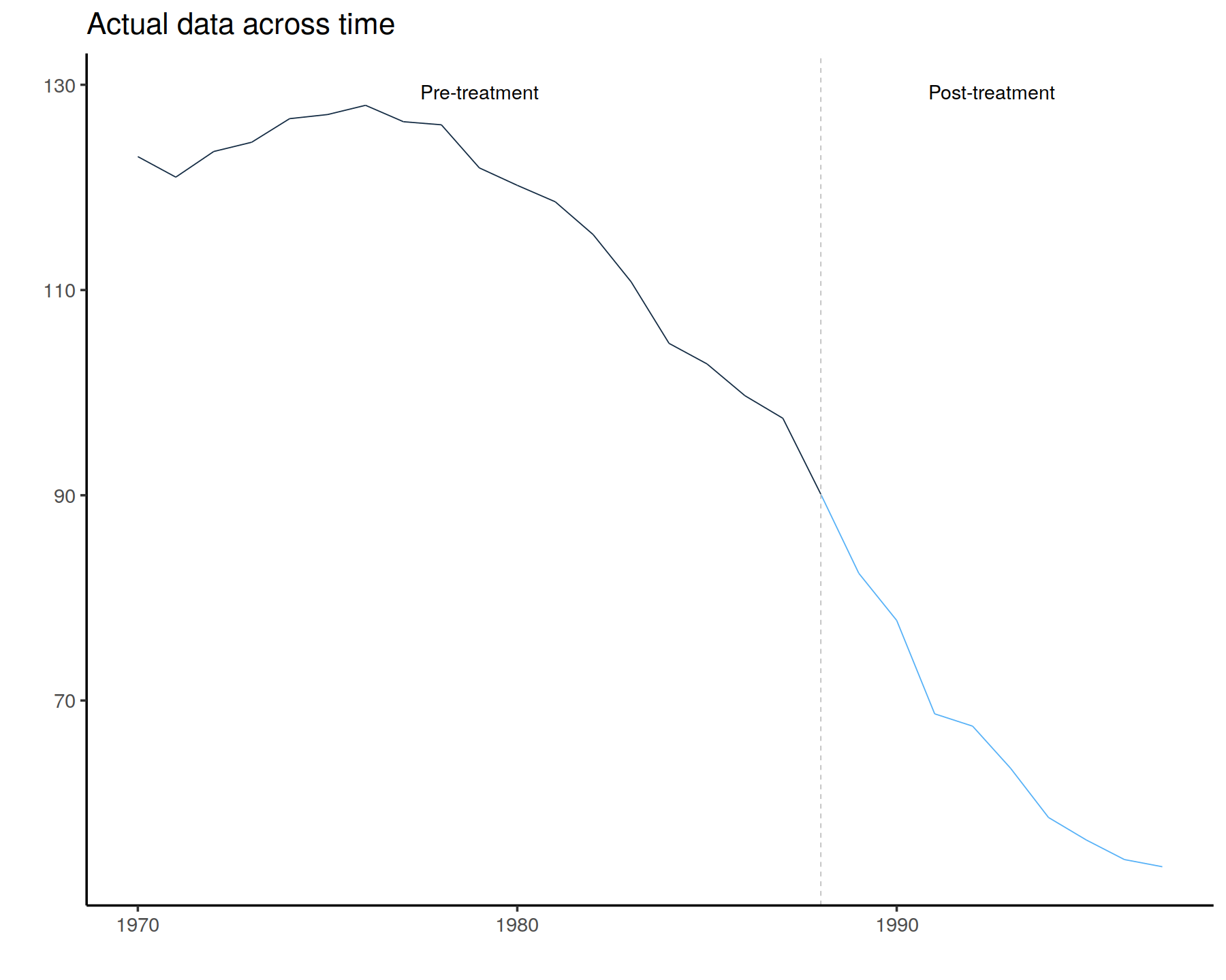
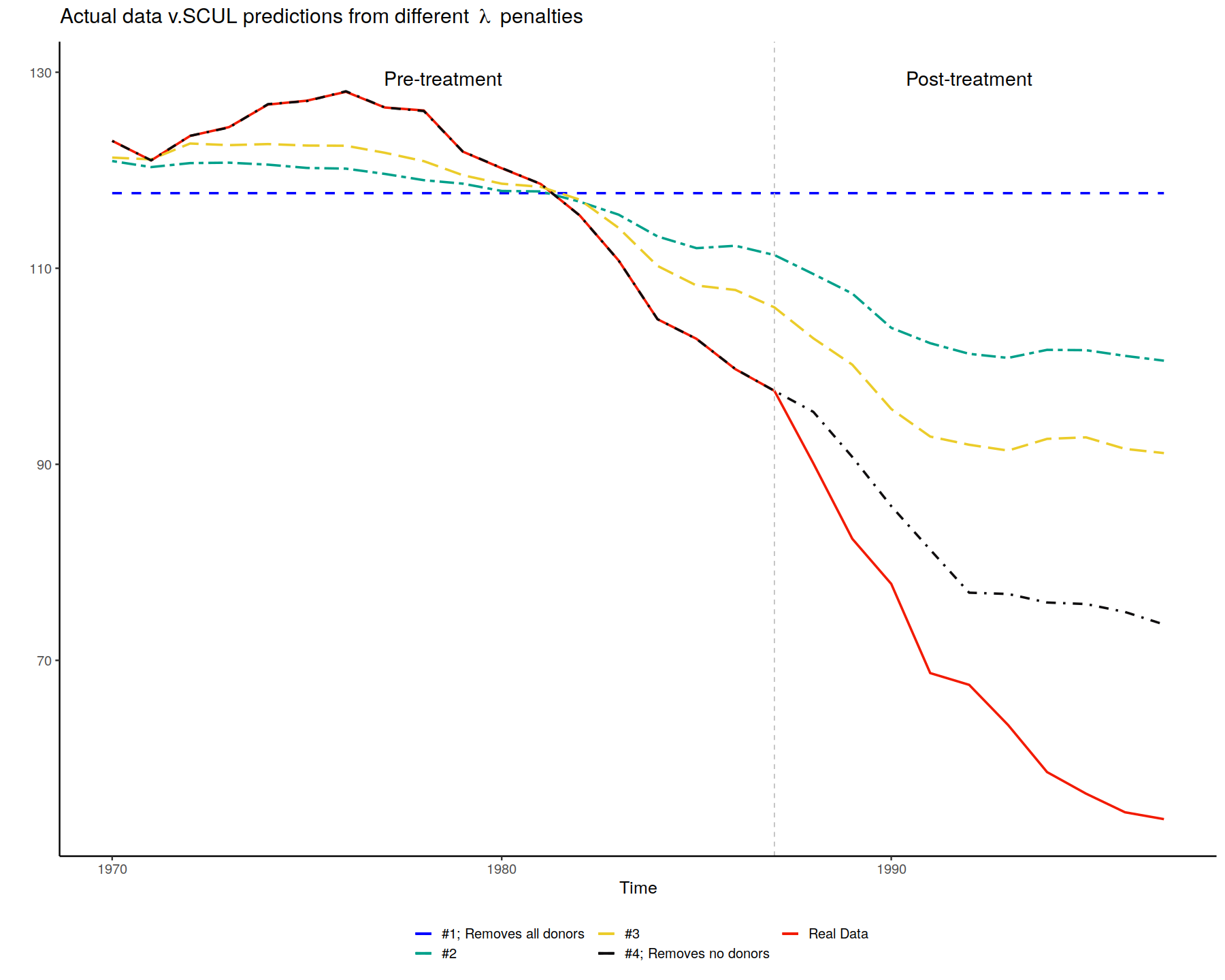
lasso_plot <-
ggplot() +
geom_line(data = data_to_plot_scul_vary_lambda,
aes(x = time, y = actual_y, color="Real Data"), size=1, linetype="solid") +
geom_line(data = data_to_plot_scul_vary_lambda,
aes(x = time, y = naive_prediction_1, color = "#1; Removes all donors"), size=1, linetype="dashed") +
geom_line(data = data_to_plot_scul_vary_lambda,
aes(x = time, y = naive_prediction_2, color="#2"), size = 1, linetype="twodash") +
geom_line(data = data_to_plot_scul_vary_lambda, aes(x = time, y = naive_prediction_3,color = "#3"), size = 1, linetype = "longdash") +
geom_line(data = data_to_plot_scul_vary_lambda, aes(x = time, y = naive_prediction_4,color = "#4; Removes no donors"), size = 1, linetype="dotdash") +
scale_color_manual(name = "",
values = c("#1; Removes all donors" = "blue", "Real Data" = "#F21A00", "#2" = "#00A08A", "#3" = "#EBCC2A", "#4; Removes no donors" = "#0F0D0E")) +
theme_bw(base_size = 15) +
theme(
panel.border = element_blank(),
panel.grid.major = element_blank(),
panel.grid.minor = element_blank(),
axis.line = element_line(colour = "black")) +
geom_vline(xintercept = data_to_plot_scul_vary_lambda$time[TreatmentBeginsAt-1], colour="grey", linetype = "dashed") + theme(legend.position="bottom") +
ylab("") +
xlab("Time") +
ggtitle(expression("Actual data v.SCUL predictions from different"~lambda~"penalties")) +
annotate("text", x = (data_to_plot_scul_vary_lambda$time[TreatmentBeginsAt-1]-data_to_plot_scul_vary_lambda$time[1])/2+data_to_plot_scul_vary_lambda$time[1], y = max(data_to_plot_scul_vary_lambda[,-1])*1.01, label = "Pre-treatment",cex=6) +
annotate("text", x = (data_to_plot_scul_vary_lambda$time[nrow(SCUL.input$y)] - data_to_plot_scul_vary_lambda$time[TreatmentBeginsAt-1])/2+data_to_plot_scul_vary_lambda$time[TreatmentBeginsAt-1], y = max(data_to_plot_scul_vary_lambda[,-1])*1.01, label = "Post-treatment",cex=6) +
guides(color=guide_legend(ncol=3))
lasso_plot
In [31]:
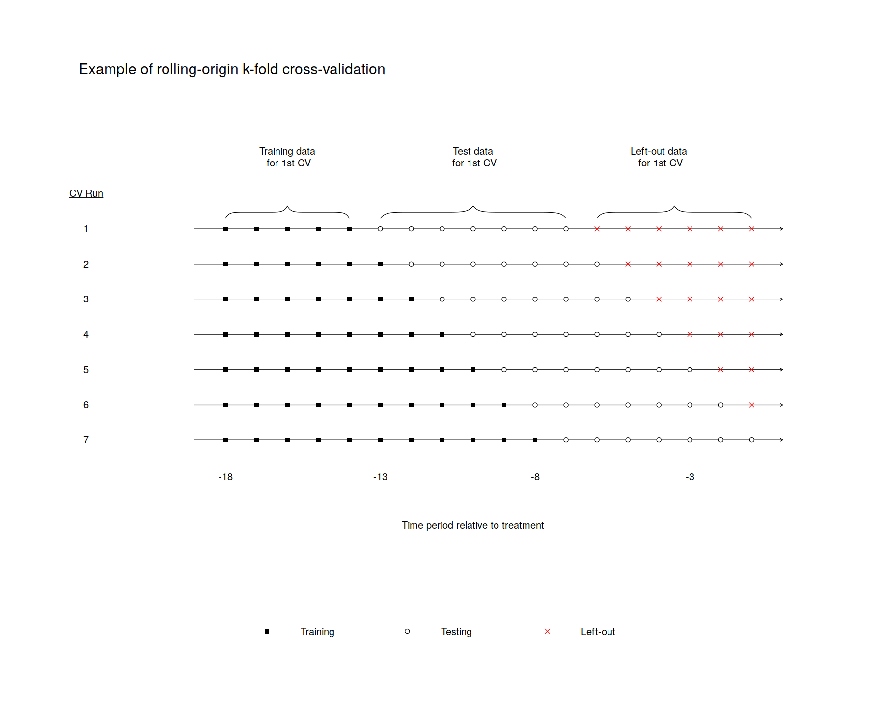
TrainingPostPeriodLength <- 7
  # Calculate the maximum number of possible runs given the previous three choices
  MaxCrossValidations <- PrePeriodLength-NumberInitialTimePeriods-TrainingPostPeriodLength+1

  # Set up the limits of the plot and astetics. (spelling?)
  plot(0,0,xlim=c(-3.75,PrePeriodLength+2.5),ylim=c(-.75,1.5),
       xaxt="n",yaxt="n",bty="n",xlab="",ylab="",type="n")

  # Set colors (train, test, left-out)
  # From Darjeeling Limited color palette, https://github.com/karthik/wesanderson
  #custom_colors <- c("#F98400", "#00A08A", "#5BBCD6")
  CustomColors <- c("black", "white", "red")
  # Loop through all the possible cross validations
  for(j in 1:MaxCrossValidations)
  {
    # Identify the possible set of test data: From one after the training data ends until the end of the pre-treatment period.
    RangeOfFullSetOfTestData <- (NumberInitialTimePeriods+j):PrePeriodLength #7:20

    # Identify the actual set of test data: From one after the training data ends until the end of test data
    RangeOfjthTestData <- (NumberInitialTimePeriods+j):(NumberInitialTimePeriods+j+TrainingPostPeriodLength-1)

    # Identify the actual set of data left out: From one after the test data ends until the end of pre-treatment data
    RangeOfLeftoutData <- (NumberInitialTimePeriods+j+TrainingPostPeriodLength):PrePeriodLength

    #  Identify the training data. From the first one until adding (J-1).
    RangeOfTrainingData <- 1:(NumberInitialTimePeriods-1+j)

    # Put arrows through the data points to represent time
    arrows(0,1-j/MaxCrossValidations,PrePeriodLength+1,1-j/MaxCrossValidations,0.05)

    # Add squares to all of the training data
    points(RangeOfTrainingData,rep(1-j/MaxCrossValidations,length(RangeOfTrainingData)),pch=15,col=CustomColors[1])

    # Add X's to the unused data
    if(length(RangeOfFullSetOfTestData) > TrainingPostPeriodLength)
      points(RangeOfLeftoutData, rep(1-j/MaxCrossValidations,length(RangeOfLeftoutData)), pch=4, col=CustomColors[3])

    # Add circles to the test data
    if(length(RangeOfFullSetOfTestData) >= TrainingPostPeriodLength)
      points(RangeOfjthTestData,rep(1-j/MaxCrossValidations,length(RangeOfjthTestData)), pch=21, col="black",bg=CustomColors[2])
  }
  # Add informative text and bracket

  ## label what is training data
  brackets(1, .9 , NumberInitialTimePeriods, .9, h=.05)
  text((NumberInitialTimePeriods+1)/2,1.15,"Training data\n for 1st CV")

  ## label what is test data
  brackets((NumberInitialTimePeriods+1), .9 , (NumberInitialTimePeriods+TrainingPostPeriodLength), .9, h=.05)
  text((NumberInitialTimePeriods+TrainingPostPeriodLength)-((TrainingPostPeriodLength-1)/2),1.15,"Test data\n for 1st CV")

  ## label what is left-out data
  brackets(NumberInitialTimePeriods+TrainingPostPeriodLength+1, .9 , PrePeriodLength, .9, h=.05)
  text((PrePeriodLength-(PrePeriodLength-NumberInitialTimePeriods-TrainingPostPeriodLength)/2),1.15,"Left-out data\n for 1st CV")


  ## Add a legend so it will be clear in black and white

  legend(
    x="bottom",
    legend=c("Training", "Testing","Left-out"),
    bg=CustomColors,
    col=c(CustomColors[1], "black", CustomColors[3]),
    lwd=1,
    lty=c(0,0),
    pch=c(15,21,4),
    bty="n",
    horiz = TRUE,
    x.intersp=.5,
    y.intersp= .25 ,
    text.width=c(2.5,2.5,2.5)
  )

  # Add custom x-axis labels to indicate time until treatment
  text(PrePeriodLength/2,-.35,"Time period relative to treatment", cex=1)
  CustomXLables <-seq((-PrePeriodLength),0, by=1)
  for (z in seq(from = 1, to = PrePeriodLength + 1, by=5)) {
    text(z, -.15, CustomXLables[z], cex=1)
  }

  # Add custom y-axis labels to indicate CV run number
  text(-3.5,1,bquote(underline("CV Run")), cex=1)
  for (z in seq(from = 0, to = 1-1/MaxCrossValidations, by = (1/MaxCrossValidations))) {
    TempLabel = MaxCrossValidations - z*MaxCrossValidations
    text(-3.5,z,TempLabel, cex=1)
  }

# Add title
#title(main = "Example of rolling origin cross-validation procedure",line = -.8)
text(-3.75, 1.5, "Example of rolling-origin k-fold cross-validation",cex=1.5,adj=0)

dev.off()
In [33]:
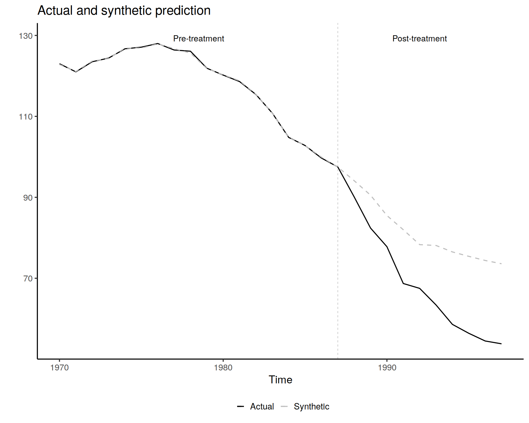
SCUL.output <- SCUL()


## ---- fig.height=8, fig.width=12, warning = FALSE, fig.align = "center", out.width = '100%'----
PlotActualvSCUL()
In [34]:
## ---- echo = FALSE------------------------------------------------------------
# Calculate pre-treatment sd
PreTreatmentSD <- sd(unlist(SCUL.output$y.actual[1:(SCUL.input$TreatmentBeginsAt-1),]))

# Store Cohen's D in each period for cross-validated lambda
StandardizedDiff <- abs(SCUL.output$y.actual-SCUL.output$y.scul)/PreTreatmentSD
names(StandardizedDiff) <- c("scul.cv")

# Store Cohen's D in each period for max lambda
StandardizedDiff$naive_prediction_1 <- abs(data_to_plot_scul_vary_lambda$naive_prediction_1 - data_to_plot_scul_vary_lambda$actual_y)/PreTreatmentSD
StandardizedDiff$naive_prediction_2 <- abs(data_to_plot_scul_vary_lambda$naive_prediction_2 - data_to_plot_scul_vary_lambda$actual_y)/PreTreatmentSD
StandardizedDiff$naive_prediction_3 <- abs(data_to_plot_scul_vary_lambda$naive_prediction_3 - data_to_plot_scul_vary_lambda$actual_y)/PreTreatmentSD
StandardizedDiff$naive_prediction_4 <- abs(data_to_plot_scul_vary_lambda$naive_prediction_4 - data_to_plot_scul_vary_lambda$actual_y)/PreTreatmentSD

# Show Cohen's D for each of these
CohensD <- data.frame(colMeans(StandardizedDiff[1:(TreatmentBeginsAt-1),]))


# Calculate treatment effect for each of these

TreatmentEffect <- SCUL.output$y.actual-SCUL.output$y.scul
names(TreatmentEffect) <- c("scul.cv")

TreatmentEffect$naive_prediction_1 <-
  data_to_plot_scul_vary_lambda$actual_y -
  data_to_plot_scul_vary_lambda$naive_prediction_1
TreatmentEffect$naive_prediction_2 <-
  data_to_plot_scul_vary_lambda$actual_y -
  data_to_plot_scul_vary_lambda$naive_prediction_2
TreatmentEffect$naive_prediction_3 <-
  data_to_plot_scul_vary_lambda$actual_y-
  data_to_plot_scul_vary_lambda$naive_prediction_3
TreatmentEffect$naive_prediction_4 <-
  data_to_plot_scul_vary_lambda$actual_y -
  data_to_plot_scul_vary_lambda$naive_prediction_4


AvgTreatmentEffect <- data.frame(colMeans(TreatmentEffect[TreatmentBeginsAt:nrow(StandardizedDiff),]))

# For target variable
Results.y.CohensD <- SCUL.output$CohensD
Results.y.StandardizedDiff <- (SCUL.output$y.actual-SCUL.output$y.scul)/sd(unlist(SCUL.output$y.actual[1:(SCUL.input$TreatmentBeginsAt-1),]))
Results.y <- SCUL.output$y.scul


## ---- echo = FALSE, warning = FALSE, message=FALSE----------------------------
table_for_hux <- cbind(
  (CohensD),
  (AvgTreatmentEffect)
)
names(table_for_hux) <- c("CohensD", "ATE")

table_for_hux$name <- c("Cross-validation for determining penalty", "Naive guess 1:\n Max penalty (remove all donors)", "Naive guess 2:\n Random penalty", "Naive guess 3:\n Random penalty", "Naive guess 4:\n No penalty (include all donors)")
table_for_hux$value <- c(SCUL.output$CrossValidatedLambda, first_guess_lasso$lambda[1], first_guess_lasso$lambda[round(length(first_guess_lasso$lambda)/10)], first_guess_lasso$lambda[round(length(first_guess_lasso$lambda)/5)], 0)

table_for_hux <- table_for_hux[c(3, 4, 1,2)]
In [36]:
libreq(IRdisplay)
In [37]:
kable(table_for_hux, col.names = c("Method","Penalty parameter", "Cohens D (pre-period fit)", "ATE estimate"), digits = 2, row.names = FALSE) %>%
  kable_styling(bootstrap_options = "striped", full_width = F) %>%
column_spec(1, width = "5cm") %>%
column_spec(2:4, width = "2cm")  %>%
  pack_rows("SCUL procedure using:", 1, 1) %>%
  pack_rows("SCUL using naive guesses for penalty", 2, 5) %>%
    as.character() %>%
    display_html()
In [38]:
PlotShareTable()
In [40]:
drop_vars_from_same_FIPS <-
 "select(-ends_with(substring(names(x.PlaceboPool)[h],nchar(names(x.PlaceboPool)[h]) - 2 + 1, nchar(names(x.PlaceboPool)[h]))))"

## ---- results='hide'----------------------------------------------------------
SCUL.inference <- CreatePlaceboDistribution(
  DonorPoolRestrictionForEachPlacebo = drop_vars_from_same_FIPS
)
In [41]:
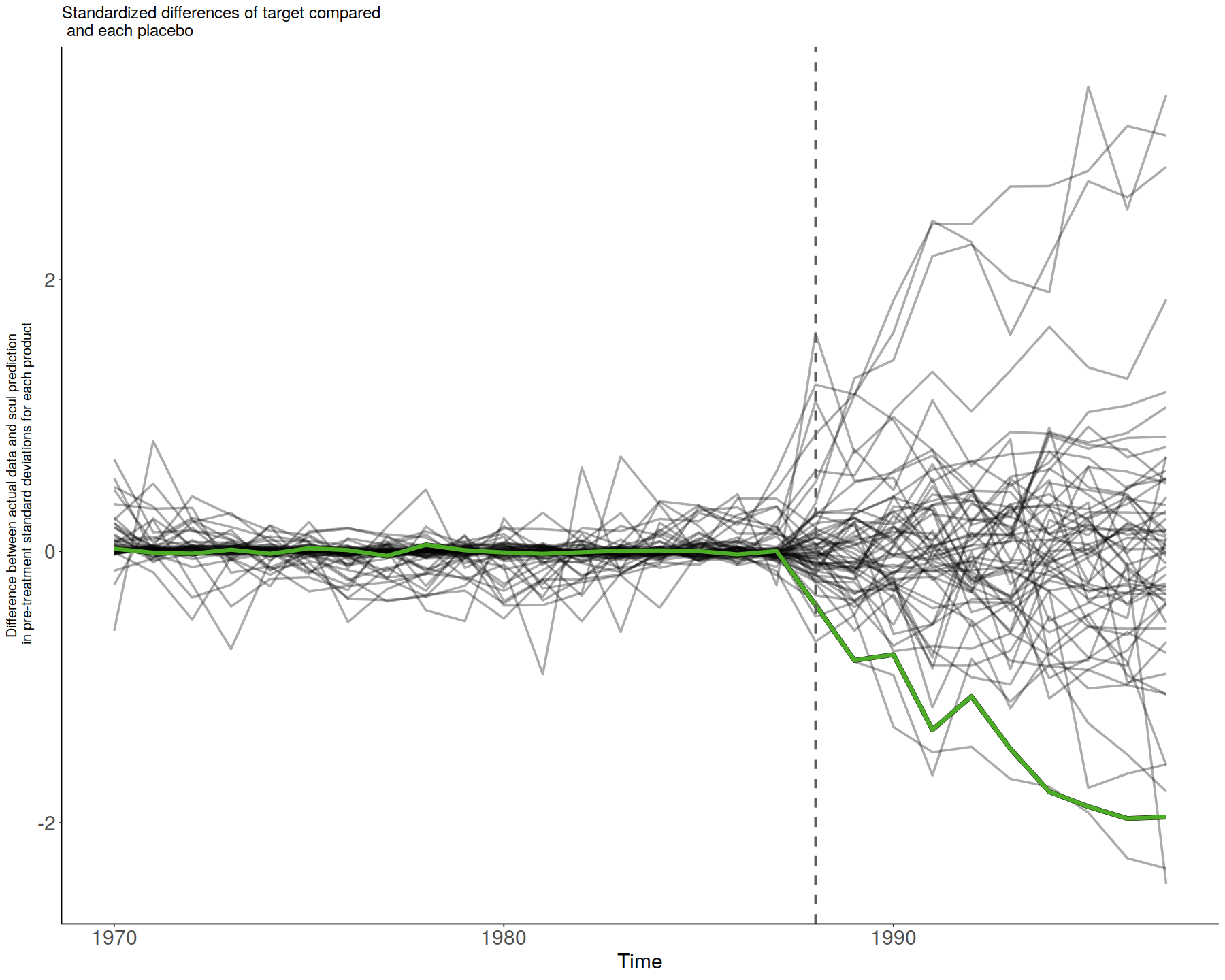
smoke_plot <- SmokePlot()
smoke_plot
In [42]:
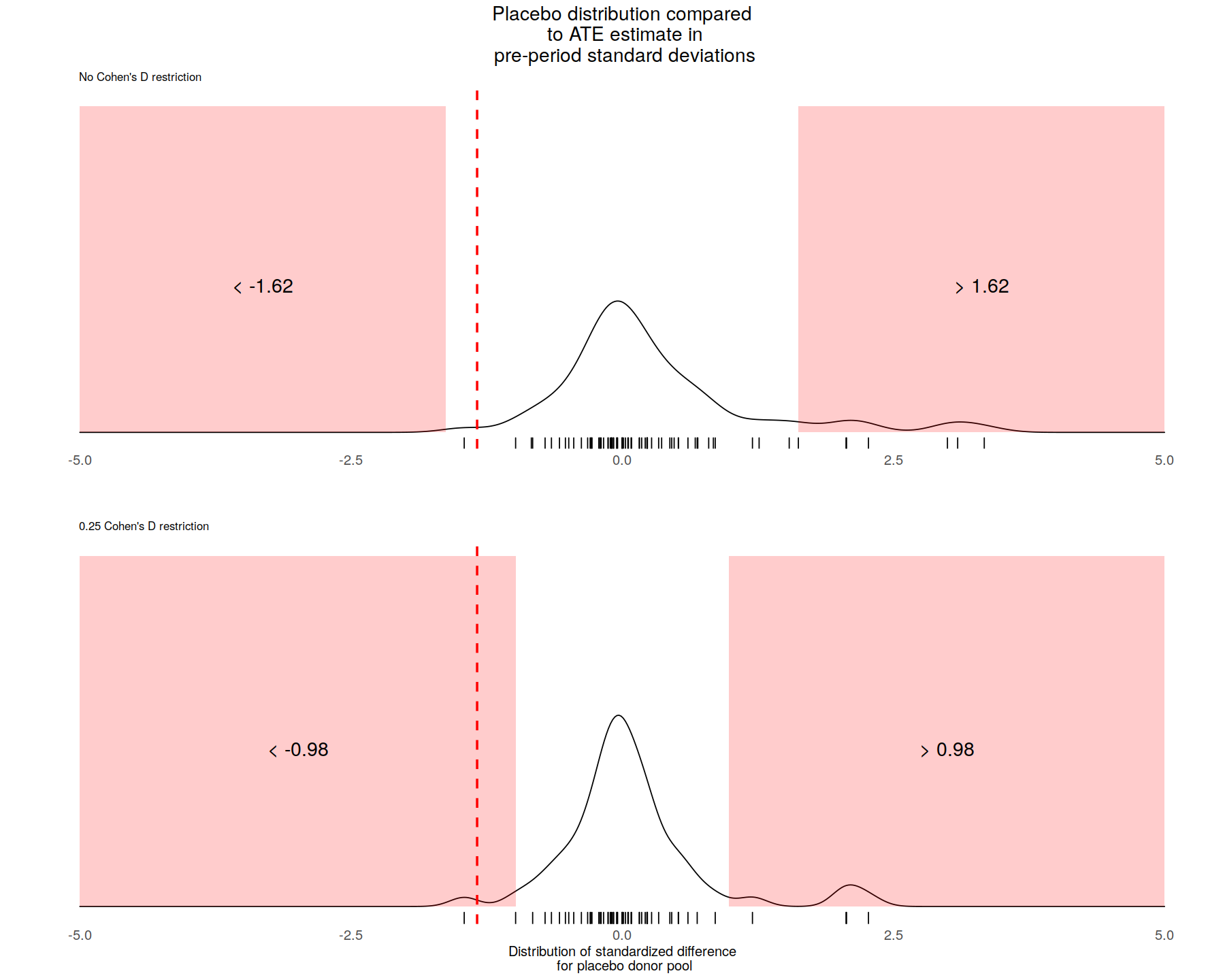
# Plot null distribution with no restriction on pre-period fit
NullDist.Full <- PlotNullDistribution(
    CohensD = 999,
    StartTime = TreatmentBeginsAt,
    EndTime = nrow(SCUL.output$y.actual),
    height = 2,
    AdjustmentParm = 1,
    BandwidthParm = .25,
    title_label = "Placebo distribution compared\n to ATE estimate in\n pre-period standard deviations",
    y_label  = " ",
    x_label  =  "",
    subtitle_label  =  "No Cohen's D restriction",
    rejection_label  =  ""
) +
  geom_vline(
        xintercept = mean(Results.y.StandardizedDiff[TreatmentBeginsAt:nrow(Results.y.StandardizedDiff),]),
        linetype = "dashed",
        size = 1,
        color = "red")

# Plot null distribution 0.25 cohen's D restriction on pre-period fit
NullDist.25 <- PlotNullDistribution(
    CohensD = 0.25,
    StartTime = TreatmentBeginsAt,
    EndTime = nrow(SCUL.output$y.actual),
    height = 2,
    AdjustmentParm = 1,
    BandwidthParm = .25,
    y_label  = "",
    x_label  =  "Distribution of standardized difference\n for placebo donor pool",
    subtitle_label  =  "0.25 Cohen's D restriction",
    rejection_label  =  "",
    title_label = " ",

) +
  geom_vline(
        xintercept = mean(Results.y.StandardizedDiff[TreatmentBeginsAt:nrow(Results.y.StandardizedDiff),]),
        linetype = "dashed",
        size = 1,
        color = "red")

# Plot n
# Combine the three plots
combined_plot <- plot_grid(
    NullDist.Full,NullDist.25,
    ncol = 1)

# Display the plot
combined_plot
In [43]:
## -----------------------------------------------------------------------------
#########################################################################################################
# Calculate an average post-treatment p-value
PValue(
    CohensD = 999,
    StartTime = SCUL.input$TreatmentBeginsAt,
    EndTime = nrow(Results.y.StandardizedDiff)
)

PValue(
    CohensD = .25,
    StartTime = SCUL.input$TreatmentBeginsAt,
    EndTime = nrow(Results.y.StandardizedDiff)
)
In [44]:
data_for_traditional_scm <- pivot_longer(data = cigarette_sales,
                                  cols = starts_with(c("cigsale_", "retprice_")),
   names_to = c("variable", "fips"),
   names_sep = "_",
   names_prefix = "X",
   values_to = "value",
   values_drop_na = TRUE
 )

data_for_traditional_scm <- pivot_wider(data = data_for_traditional_scm,
                                  names_from = variable,
                                  values_from = value)


 data_for_traditional_scm$fips <- as.numeric(data_for_traditional_scm$fips)
In [45]:
data(synth.data)

# create matrices from panel data that provide inputs for synth()
data_for_traditional_scm$idno = as.numeric(as.factor(data_for_traditional_scm$fips))  # create numeric country id required for synth()

data_for_traditional_scm <- as.data.frame(data_for_traditional_scm)

dataprep.out<-
  dataprep(
    foo = data_for_traditional_scm,
    predictors = c("retprice"),
    predictors.op = "mean",
    dependent = "cigsale",
    unit.variable = "idno",
    time.variable = "year",
    special.predictors = list(
      list("cigsale", 1970, "mean"),
      list("cigsale", 1980, "mean"),
      list("cigsale", 1985, "mean")
    ),
    treatment.identifier = unique(data_for_traditional_scm$idno[data_for_traditional_scm$fips==6]),
    controls.identifier = unique(data_for_traditional_scm$idno[data_for_traditional_scm$fips!=6]),
    time.predictors.prior = c(1970:1987),
    time.optimize.ssr = c(1970:1987),
    time.plot = 1970:1997
  )

## run the synth command to identify the weights
## that create the best possible synthetic
## control unit for the treated.
synth.out <- synth(dataprep.out)
In [46]:
gaps<- dataprep.out$Y1plot-(
  dataprep.out$Y0plot%*%synth.out$solution.w
)

StandardizedDiff$traditional_scm <- abs(dataprep.out$Y1plot-(
  dataprep.out$Y0plot%*%synth.out$solution.w
))/PreTreatmentSD

# Show Cohen's D for each of these
CohensD <- data.frame(colMeans(StandardizedDiff[1:(TreatmentBeginsAt-1),]))


# Calculate treatment effect for each of these
TreatmentEffect <- data.frame(colMeans(StandardizedDiff[TreatmentBeginsAt:nrow(StandardizedDiff),])*PreTreatmentSD)
In [47]:
StandardizedDiff<-cbind(StandardizedDiff,SCUL.input$time)
colnames(StandardizedDiff)[7] <- "time"
# create smoke plot
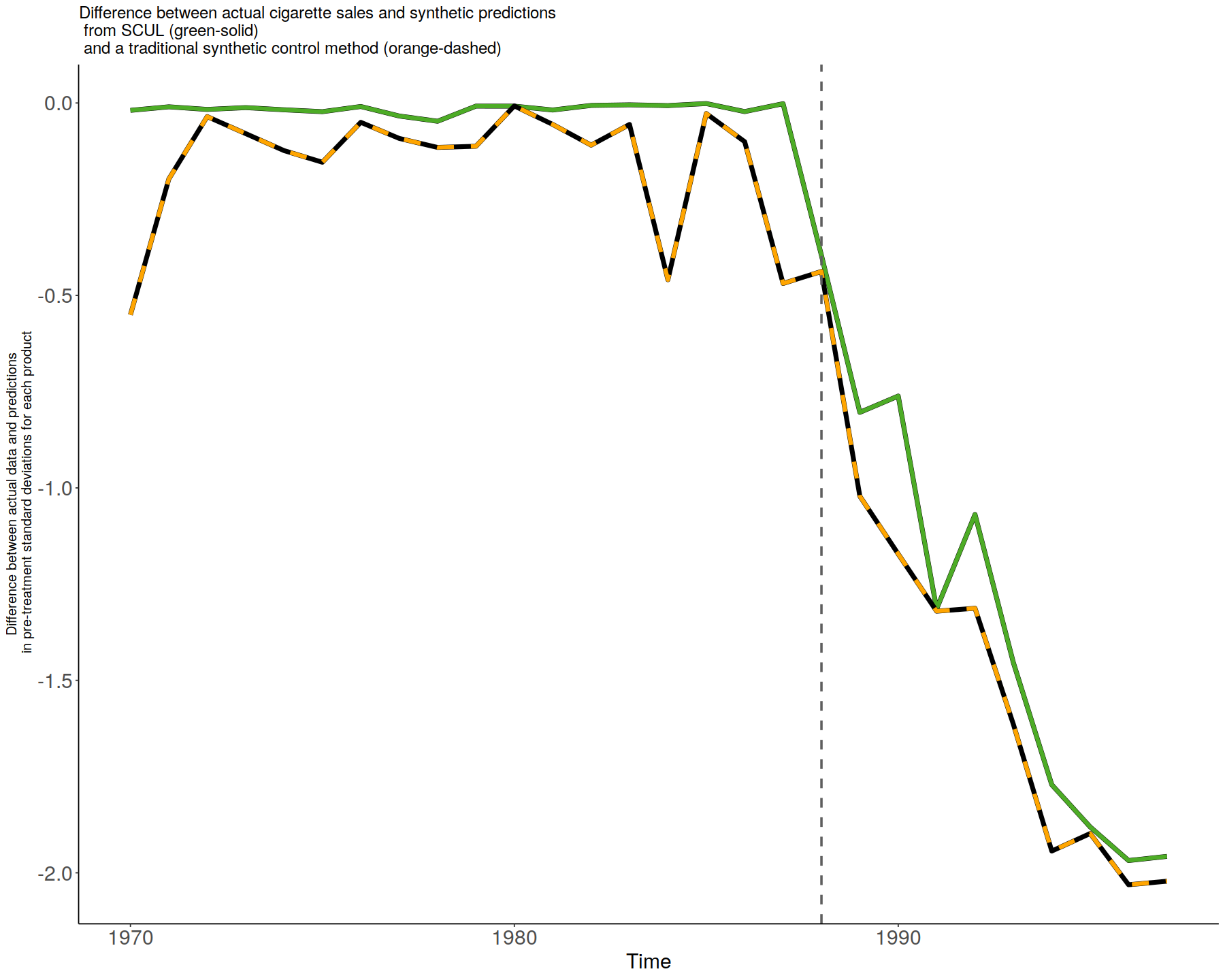
difference_plot <- ggplot() +
theme_classic() +
geom_line(data = StandardizedDiff, aes(x = time, y = -scul.cv), alpha = 1, size = 2., color = "black") +
geom_line(data = StandardizedDiff, aes(x = time, y = -scul.cv), alpha = 1, size = 1.75, color = "#4dac26") +
geom_line(data = StandardizedDiff, aes(x = time, y = -traditional_scm), alpha = 1, size = 2., color = "black") +
geom_line(data = StandardizedDiff, aes(x = time, y = -traditional_scm), alpha = 1, size = 1.75, color = "orange", linetype = "dashed") +
geom_vline(
xintercept = SCUL.input$time[TreatmentBeginsAt,1],
linetype = "dashed",
size = 1,
color = "grey37"
) +
labs(
title = "Difference between actual cigarette sales and synthetic predictions\n from SCUL (green-solid)\n and a traditional synthetic control method (orange-dashed)",
x = "Time",
y = "Difference between actual data and predictions\n in pre-treatment standard deviations for each product"
) +
theme(
axis.text = element_text(size = 18),
axis.title.y = element_text(size = 12),
axis.title.x = element_text(size = 18),
title = element_text(size = 12)
)
# Display graph
difference_plot
In [48]:
table_for_hux_scm <- cbind(
  (CohensD),
  (TreatmentEffect)
)
table_for_hux_scm <- table_for_hux_scm[-(2:5),]

names(table_for_hux_scm) <- c("CohensD", "ATE")

table_for_hux_scm$name <- c("Cross-validation for determining penalty", " ")
table_for_hux_scm$value <- c(round(SCUL.output$CrossValidatedLambda, digits = 2), "NA")

table_for_hux_scm <- table_for_hux_scm[c(3, 4, 1,2)]


kable(table_for_hux_scm, col.names = c("Method","Penalty parameter", "Cohens D (pre-period fit)", "ATE estimate"), digits = 3, row.names = FALSE) %>%
  kable_styling(bootstrap_options = "striped", full_width = F) %>%
column_spec(1, width = "5cm") %>%
column_spec(2:4, width = "2cm")  %>%
  pack_rows("SCUL procedure using:", 1, 1) %>%
  pack_rows("Traditional SCM method", 2, 2) %>% as.character %>% display_html
In [ ]: