Staggered DiD framework (Callaway and Sant'anna)
$\newcommand{\defeq}{:=}$ $\newcommand{\var}{\mathrm{Var}}$ $\newcommand{\epsi}{\varepsilon}$ $\newcommand{\phii}{\varphi}$ $\newcommand\Bigpar[1]{\left( #1 \right )}$ $\newcommand\Bigbr[1]{\left[ #1 \right ]}$ $\newcommand\Bigcr[1]{\left\{ #1 \right \}}$ $\newcommand\SetB[1]{\left\{ #1 \right\}}$ $\newcommand\Sett[1]{\mathcal{#1}}$ $\newcommand{\Data}{\mathcal{D}}$ $\newcommand{\Ubr}[2]{\underbrace{#1}_{\text{#2}}}$ $\newcommand{\Obr}[2]{ \overbrace{#1}^{\text{#2}}}$ $\newcommand{\sumiN}{\ensuremath{\sum_{i=1}^N}}$ $\newcommand{\dydx}[2]{\frac{\partial #1}{\partial #2}}$ $\newcommand{\Realm}[1]{\mathbb{R}^{#1}}$ $\newcommand{\Exp}[1]{\mathbb{E}\left[#1\right]}$ $\newcommand{\Expt}[2]{\mathbb{E}_{#1}\left[#2\right]}$ $\newcommand{\Var}[1]{\mathbb{V}\left[#1\right]}$ $\newcommand{\Covar}[1]{\text{Cov}\left[#1\right]}$ $\newcommand{\Prob}[1]{\mathbf{Pr}\left(#1\right)}$ $\newcommand{\Supp}[1]{\text{Supp}\left[#1\right]}$ $\newcommand{\doyx}{\Prob{Y \, |\,\mathsf{do} (X = x)}}$ $\newcommand{\doo}[1]{\Prob{Y |\,\mathsf{do} (#1) }}$ $\newcommand{\R}{\ensuremath{\mathbb{R}}}$ $\newcommand{\Z}{\ensuremath{\mathbb{Z}}}$ $\newcommand{\wh}[1]{\widehat{#1}} % Wide hat$ $\newcommand{\wt}[1]{\widetilde{#1}} % Wide tilde$ $\newcommand{\wb}[1]{\overline{#1}} % Wide bar$ $\newcommand\Ol[1]{\overline{#1}}$ $\newcommand\Ul[1]{\underline{#1}}$ $\newcommand\Str[1]{#1^{*}}$ $\newcommand{\F}{\mathsf{F}}$ $\newcommand{\ff}{\mathsf{f}}$ $\newcommand{\Cdf}[1]{\mathbb{F}\left(#1\right)}$ $\newcommand{\Cdff}[2]{\mathbb{F}_{#1}\left(#2\right)}$ $\newcommand{\Pdf}[1]{\mathsf{f}\left(#1\right)}$ $\newcommand{\Pdff}[2]{\mathsf{f}_{#1}\left(#2\right)}$ $\newcommand{\dd}{\mathsf{d}}$ $\newcommand\Normal[1]{\mathcal{N} \left( #1 \right )}$ $\newcommand\Unif[1]{\mathsf{U} \left[ #1 \right ]}$ $\newcommand\Bern[1]{\mathsf{Bernoulli} \left( #1 \right )}$ $\newcommand\Binom[1]{\mathsf{Bin} \left( #1 \right )}$ $\newcommand\Pois[1]{\mathsf{Poi} \left( #1 \right )}$ $\newcommand\BetaD[1]{\mathsf{Beta} \left( #1 \right )}$ $\newcommand\Diri[1]{\mathsf{Dir} \left( #1 \right )}$ $\newcommand\Gdist[1]{\mathsf{Gamma} \left( #1 \right )}$ $\def\mbf#1{\mathbf{#1}}$ $\def\mrm#1{\mathrm{#1}}$ $\def\mbi#1{\boldsymbol{#1}}$ $\def\ve#1{\mbi{#1}} % Vector notation$ $\def\vee#1{\mathbf{#1}} % Vector notation$ $\newcommand{\Mat}[1]{\mathbf{#1}}$ $\newcommand{\eucN}[1]{\norm{#1}}$ $\newcommand{\lzero}[1]{\norm{#1}_0}$ $\newcommand{\lone}[1]{\norm{#1}_1}$ $\newcommand{\ltwo}[1]{\norm{#1}_2}$ $\newcommand{\pnorm}[1]{\norm{#1}_p}$
TWFE works when
- effects aren't heterogeneous
- 2 time perids
in a TWFE regression, units whose treatment status doesn’t change over time serve as the comparison group for units whose treatment status does change over time. With multiple time periods and variation of treatment timing, some of these comparisons are:
newly treated units relative to ``never treated’’ units (good!)
newly treated units relative to ``not-yet treated’’ units (good!)
newly treated units relative to already treated units (bad!!!)
Notation
- $Y_{i t}(0)$ is unit $i$ 's untreated potential outcome. This is the outcome that unit $i$ would experience in period $t$ if they do not participate in the treatment.
- $Y_{i t}(g)$ is unit $i$ 's potential outcome in time period $t$ if they become treated in period $g$.
- $G_{i}$ is the time period when unit $i$ becomes treated (often groups are defined by the time period when a unit becomes treated; hence, the $G$ notation).
- $C_{i}$ is an indicator variable for whether unit $i$ is in a never-treated group.
- $D_{i t}$ is an indicator variable for whether unit $i$ has been treated by time $t$.
- $Y_{i t}$ is unit $i$ 's observed outcome in time period $t$. For units in the never-treated group, $Y_{i t}=Y_{i t}(0)$ in all time periods. For units in other groups, we observe $Y_{i t}=1\left\{G_{i}>t\right\} Y_{i t}(0)+\mathbf{1}\left\{G_{i} \leq t\right\} Y_{i t}\left(G_{i}\right)$. The notation here is a bit complicated, but in words, we observe untreated potential outcomes for units that have not yet participated in the treatment, and we observe treated potential outcomes for units once they start to participate in the treatment (and these can depend on when they became treated).
- $\ve{X}_i$ is a vector of pretreatment covariates
Assumptions:
- Staggered Treatment Adoption Assumption
- Parallel trends assumption based on never treated units
- Parallel trends assumption based on not-yet-treated units
Estimands:
Group-time average treatment effects
$$ ATT(g, t) = \Exp{Y_t(g) - Y_t(0)|G = g} $$Aggregated into ATE by group
$$ \theta_{S}(g)=\frac{1}{\mathcal{T}-g+1} \sum_{t=2}^{\mathcal{T}} \mathbf{1}\{g \leq t\} \operatorname{ATT}(g, t) $$Further aggregate this into an overall-effect parameter
$$ \theta_{S}^{O}:=\sum_{g=2}^{\mathcal{T}} \theta_{S}(g) P(G=g) $$Treatment effect dynamics
$$ \theta_{D}(e):=\sum_{g=2}^{\mathcal{T}} 1\{g+e \leq \mathcal{T}\} A T T(g, g+e) P(G=g \mid G+e \leq \mathcal{T}) $$where $e$ is the number of periods that a unit has been exposed to treatment
rm(list = ls())
library(LalRUtils)
libreq(data.table, magrittr, tidyverse, janitor, stargazer2, patchwork,
       knitr, IRdisplay, rlist, fixest)
theme_set(lal_plot_theme()) # add _d() for dark
set.seed(42)
options(repr.plot.width = 8, repr.plot.height=6)
chr = function(...) as.character(...)
#%%
libreq(DIDmultiplegt, did, bacondecomp, PanelMatch, panelView, gsynth, tictoc)
Simulated data
Model for untreated potential outcomes $$ Y_{it}(0) = \theta_t + \eta_i + \ve{X_i}' \beta_t + v_{it} $$
treated potential outcome
$$ Y_{it}(g) = Y_{it}(0) + 1 \Bigpar{t \geq g} (e + 1) + \epsi_{it} - v_{it} $$where $e \defeq t - g$, i.e. the treatment effect is the event time.
- $\theta_{t}=\beta_{t}=t$ for $t=1, \ldots, 4$
- $\eta_{i} \sim N\left(G_{i}, 1\right)$ where $G_{i}$ is which group an individual belongs to,
- $X_{i} \sim N\left(\mu_{D_{i}}, 1\right)$ where $\mu_{D_{i}}=1$ for never treated units and 0 otherwise
- $v_{i t} \sim N(0,1),$ and $u_{i t} \sim N(0,1)$
- Also, all random variables are drawn independently of each other.
reset.sim <- function() {
  #-----------------------------------------------------------------------------
  # set parameters
  #-----------------------------------------------------------------------------
  # number of time periods
  # time.periods <<- 4
  # number of treated units
  nt <<- 4000
  # coefficient on X
  bett <<- seq(1:time.periods)
  # time fixed effect
  thet <<- seq(1:time.periods)
  # number of untreated units
  nu <<- 4000
  # time fixed effect
  theu <<- thet # changing this creates violations of parallel trends
  # covariate effect
  betu <<- bett # changing this creates violations of conditional parallel trends
  #-----------------------------------------------------------------------------
  # parameters for treated potential outcomes
  #-----------------------------------------------------------------------------
  te.bet.ind <<- rep(1,time.periods) # no selective treatment timing
  te.bet.X <<- bett #no heterogeneous effects by X
  te.t <<- thet # no calendar time effects
  te.e <<- rep(0,time.periods) # no dynamic effects
  te <<- 1 # overall basic effect
  #-----------------------------------------------------------------------------
  # extra parameters for an ipw sim (otherwise, these are not used)
  #-----------------------------------------------------------------------------
#   n <<- 4000
  # these are parameters in generalized propensity score
  # don't make them too big otherwise can get divide by 0
  gamG <<- c(0,1:time.periods)/(2*time.periods)
}


build_sim_dataset <- function(panel=TRUE) {
  #-----------------------------------------------------------------------------
  # build dataset
  #-----------------------------------------------------------------------------

  # randomly assign treated units to groups
  # random groups
  G <- sample(1:time.periods, size=nt, replace=TRUE)
  # fixed groups
  # G <- unlist(lapply(1:T, function(g) rep(g, nt/T)))

  # draw a single covariate
  Xt <- rnorm(nt)

  # draw individual fixed effect
  Ct <- rnorm(nt, mean=G)

  # generate untreated potential outcomes in each time period
  Ynames <- paste0("Y",1:time.periods)
  Ynames <- paste0(1:time.periods)
  Y0tmat <- sapply(1:time.periods, function(t) {
    thet[t] + Ct + Xt*bett[t] + rnorm(nt)
  })
  Y0tdf <- as.data.frame(Y0tmat)

  # generate treated potential outcomes
  Y1tdf <- sapply(1:time.periods, function(t) {
    te.t[t] + te.bet.ind[G]*Ct + Xt*te.bet.X[t] + (G <= t)*te.e[sapply(1:nt, function(i) max(t-G[i]+1,1))] + te + rnorm(nt) # hack for the dynamic effects but ok
  })

  # generate observed data
  Ytdf <- sapply(1:time.periods, function(t) {
    (G<=t)*Y1tdf[,t] + (G>t)*Y0tdf[,t]
  })
  colnames(Ytdf) <- Ynames

  # store observed data for treated group
  dft <- cbind.data.frame(G,X=Xt,Ytdf)

  # untreated units

  # draw untreated covariate
  Xu <- rnorm(nu, mean=1)

  # draw untreated fixed effect
  Cu <- rnorm(nu)


  # generate untreated potential outcomes
  Y0umat <- sapply(1:time.periods, function(t) {
    theu[t] + Cu + rnorm(nu) + Xu*betu[t]
  })
  Y0udf <- as.data.frame(Y0umat)
  colnames(Y0udf) <- Ynames

  # store dataset of observed outcomes for untreated units
  dfu <- cbind.data.frame(G=0,X=Xu,Y0udf)

  # store overall dataset
  df <- rbind.data.frame(dft, dfu)

  # generate id variable
  df$id <- 1:nrow(df)

  # convert data from wide to long format
  library(tidyr)
  ddf <- gather(df, period, Y, -G, -X, -id)
  ddf$period <- as.numeric(ddf$period)
  ddf$treat <- 1*(ddf$G > 0)
  ddf <- ddf[order(ddf$id, ddf$period),] # reorder data

  if (!panel) { # repeated cross sections
    n <- nt+nu
    Time <- sample(1:time.periods, size=n, replace=TRUE, prob=rep(1/time.periods, time.periods))
    right.row <- sapply( unique(ddf$id), function(i) {
      which(ddf$id==i & ddf$period==Time[i])
    })
    ddf <- ddf[right.row,]
  }

  ddf <- subset(ddf, G != 1)
  ddf
}


build_ipw_dataset <- function(panel=TRUE) {

  #-----------------------------------------------------------------------------
  # build dataset
  # build things up from the generalized propensity score
  #-----------------------------------------------------------------------------
  X <- rnorm(n)

  pr <- exp(outer(X,gamG)) / apply( exp(outer(X,gamG)), 1, sum)
  GG <- apply(pr, 1, function(pvec) sample(seq(0,time.periods), size=1, prob=pvec))

  G <- GG[GG>0]
  nt <- length(G)
  Xt <- X[GG>0]

  # draw individual fixed effect
  Ct <- rnorm(nt, mean=G)

  # generate untreated potential outcomes in each time period
  Ynames <- paste0("Y",1:time.periods)
  Ynames <- paste0(1:time.periods)
  Y0tmat <- sapply(1:time.periods, function(t) {
    thet[t] + Ct + Xt*bett[t] + rnorm(nt)
  })
  Y0tdf <- as.data.frame(Y0tmat)

  # generate treated potential outcomes
  Y1tdf <- sapply(1:time.periods, function(t) {
    te.t[t] + te.bet.ind[G]*Ct + Xt*te.bet.X[t] + (G <= t)*te.e[sapply(1:nt, function(i) max(t-G[i]+1,1))] + te + rnorm(nt) # hack for the dynamic effects but ok
  })

  # generate observed data
  Ytdf <- sapply(1:time.periods, function(t) {
    (G<=t)*Y1tdf[,t] + (G>t)*Y0tdf[,t]
  })
  colnames(Ytdf) <- Ynames

  # store observed data for treated group
  dft <- cbind.data.frame(G,X=Xt,Ytdf)

  # untreated units
  nu <- n-nt

  # draw untreated covariate
  Xu <- X[GG==0]

  # draw untreated fixed effect
  Cu <- rnorm(nu)


  # generate untreated potential outcomes
  Y0umat <- sapply(1:time.periods, function(t) {
    theu[t] + Cu + rnorm(nu) + Xu*betu[t]
  })
  Y0udf <- as.data.frame(Y0umat)
  colnames(Y0udf) <- Ynames

  # store dataset of observed outcomes for untreated units
  dfu <- cbind.data.frame(G=0,X=Xu,Y0udf)

  # store overall dataset
  df <- rbind.data.frame(dft, dfu)

  # generate id variable
  df$id <- 1:nrow(df)

  # convert data from wide to long format
  library(tidyr)
  ddf <- gather(df, period, Y, -G, -X, -id)
  ddf$period <- as.numeric(ddf$period)
  ddf$treat <- 1*(ddf$G > 0)
  ddf <- ddf[order(ddf$id, ddf$period),] # reorder data

  if (!panel) { # repeated cross sections
    Time <- sample(1:time.periods, size=n, replace=TRUE, prob=rep(1/time.periods, time.periods))
    right.row <- sapply( unique(ddf$id), function(i) {
      which(ddf$id==i & ddf$period==Time[i])
    })
    ddf <- ddf[right.row,]
  }

  ddf <- subset(ddf, G != 1)

  ddf
}


sim <- function(ret=NULL, bstrap=FALSE, cband=FALSE, control.group="nevertreated",
                panel=TRUE) {

  ddf <- build_sim_dataset(panel)

  # get results
  res <- att_gt(yname="Y", xformla=~X, data=ddf, tname="period", idname="id",
                gname="G", est_method="reg",
                bstrap=bstrap, cband=cband, control_group=control.group,
                panel=panel)


  if (is.null(ret)) {
    return(res)
  } else if (ret=="Wpval") {
    rej <- 1*(res$Wpval < .05)
    return(rej)
  } else if (ret=="cband") {
    cu <- res$att + res$c * sqrt(diag(res$V))/sqrt(res$n)
    cl <- res$att - res$c * sqrt(diag(res$V))/sqrt(res$n)
    covers0 <- 1*(all( (cu > 0) & (cl < 0)))
    return(covers0)
  } else if (ret=="simple") {
    agg <- aggte(res)
    rej <- 1*( abs(agg$overall.att / agg$overall.se) > qnorm(.975) )
    return(rej)
  } else if (ret=="dynamic") {
    truth <- c(rep(0,(time.periods-2)),te+te.e[1:(time.periods-1)])
    agg <- aggte(res, type="dynamic")
    cu <- agg$att.egt + agg$crit.val.egt * agg$se.egt
    cl <- agg$att.egt - agg$crit.val.egt * agg$se.egt
    coverstruth <- 1*(all( (cu > truth) & (cl < truth)))
    return(coverstruth)
  } else if (ret=="notyettreated") {
    agg <- aggte(res)
    rej <- 1*( abs(agg$overall.att / agg$overall.se) > qnorm(.975) )
    return(rej)
  } else {
    return(res)
  }

}

pretest_sim <- function(ret=NULL, bstrap=FALSE, cband=FALSE,
                        control.group="nevertreated", panel=TRUE, xformla=~X, cores=1) {

  ddf <- build_ipw_dataset(panel=panel)

  # get results
  res <- conditional_did_pretest(yname="Y", xformla=xformla, data=ddf,
                                 tname="period", idname="id",
                                 first.treat.name="G", estMethod="ipw",
                                 printdetails=FALSE,
                                 bstrap=bstrap, cband=cband,
                                 control.group=control.group,
                                 panel=panel,
                                 pl=TRUE, cores=cores)

  res$CvMpval
}
time.periods <- 4
reset.sim()
te <- 0
# set seed so everything is reproducible
set.seed(1814)

# generate dataset with 4 time periods
time.periods <- 4

# add dynamic effects
te.e <- 1:time.periods

# generate data set with these parameters
# here, we dropped all units who are treated in time period 1 as they do not help us recover ATT(g,t)'s.
dta <- build_sim_dataset()

# How many observations remained after dropping the ``always-treated'' units
nrow(dta)
#> [1] 27952
#This is what the data looks like
head(dta)
#>       G        X id period         Y treat
#> 1     2 0.530541  1      1  4.795125     1
#> 8001  2 0.530541  1      2  7.159789     1
#> 16001 2 0.530541  1      3  8.482624     1
#> 24001 2 0.530541  1      4 11.288278     1
#> 2     4 1.123550  2      1  4.375698     1
#> 8002  4 1.123550  2      2  9.285481     1
dta = setDT(dta)
dta %>% .[, max(treat), G]
# estimate group-time average treatment effects using att_gt method
example_attgt <- att_gt(yname = "Y",
                        tname = "period",
                        idname = "id",
                        gname = "G",
                        xformla = ~X,
                        data = dta
                        )

# summarize the results
summary(example_attgt)
ggdid(example_attgt)
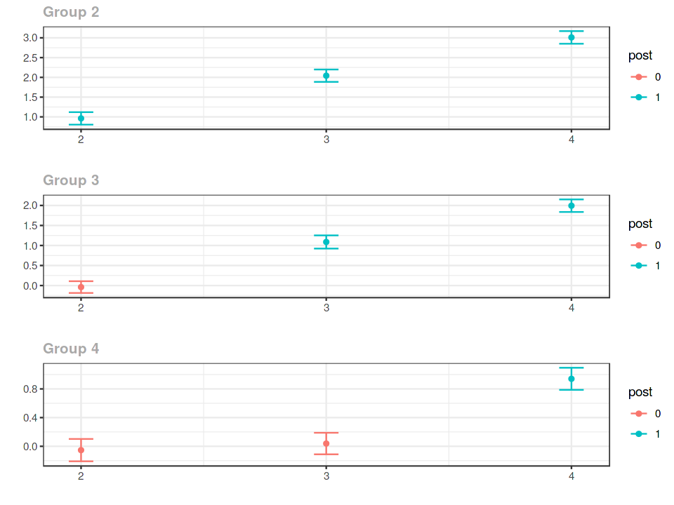
aggregation
agg.simple <- aggte(example_attgt, type = "simple")
summary(agg.simple)
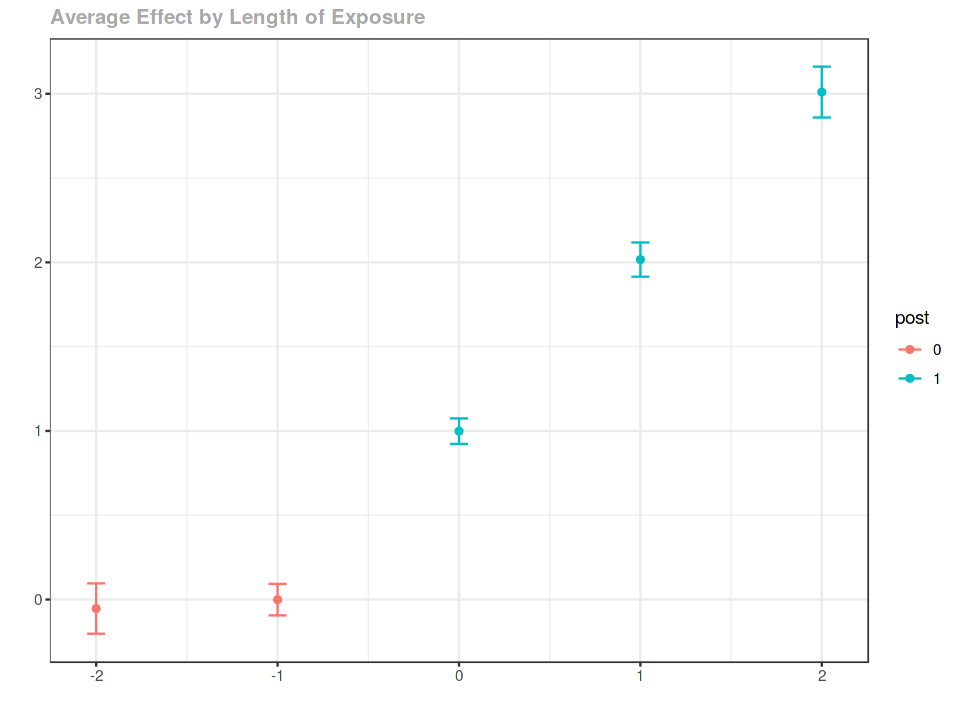
agg.es <- aggte(example_attgt, type = "dynamic")
summary(agg.es)
group effects
agg.gs <- aggte(example_attgt, type = "group")
summary(agg.gs)
Event study
ggdid(agg.es)
Using staggered design
example_attgt_altcontrol <- att_gt(yname = "Y",
                                   tname = "period",
                                   idname = "id",
                                   gname = "G",
                                   xformla = ~X,
                                   data = dta,
                                   control_group = "notyettreated"
                                   )
summary(example_attgt_altcontrol)
Data example
library(did)
data(mpdta)
mpdta %>% glimpse
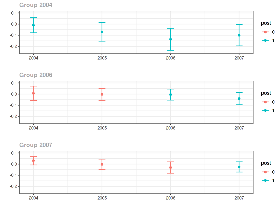
out <- att_gt(yname = "lemp",
              gname = "first.treat",
              idname = "countyreal",
              tname = "year",
              xformla = ~1,
              data = mpdta,
              est_method = "reg"
              )
out
ggdid(out, ylim = c(-.25,.1))
event study
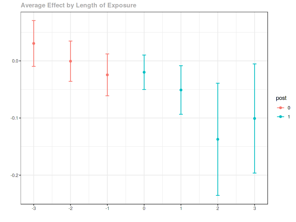
es <- aggte(out, type = "dynamic")
es %>% summary
ggdid(es)
group_effects <- aggte(out, type = "group")
summary(group_effects)