This lab on Logistic Regression in R comes from p. 161-163 of "Introduction to Statistical Learning with Applications in R" by Gareth James, Daniela Witten, Trevor Hastie and Robert Tibshirani. It was re-implemented in Fall 2016 in tidyverse format by Amelia McNamara and R. Jordan Crouser at Smith College.

4.6.3 Linear Discriminant Analysis¶

Now we will perform LDA on the Smarket data from the ISLR package. In R, we can fit a LDA model using the lda() function, which is part of the MASS library. Note: dplyr and MASS have a name clash around the word select(), so we need to do a little magic to make them play nicely.

library(MASS)
library(dplyr)
library(ISLR)
select <- dplyr::select

Attaching package: ‘dplyr’


The following object is masked from ‘package:MASS’:

    select


The following objects are masked from ‘package:stats’:

    filter, lag


The following objects are masked from ‘package:base’:

    intersect, setdiff, setequal, union

The syntax for the lda() function is identical to that of lm(), and to that of glm() except for the absence of the family option. As we did with logistic regression and KNN, we'll fit the model using only the observations before 2005, and then test the model on the data from 2005.

train = Smarket %>%
  filter(Year < 2005)

test = Smarket %>%
  filter(Year >= 2005)

model_LDA = lda(Direction~Lag1+Lag2, data = train)
print(model_LDA)

Call:
lda(Direction ~ Lag1 + Lag2, data = train)

Prior probabilities of groups:
 Down    Up 
0.492 0.508 

Group means:
         Lag1     Lag2
Down  0.04279  0.03389
Up   -0.03955 -0.03133

Coefficients of linear discriminants:
         LD1
Lag1 -0.6420
Lag2 -0.5135

The LDA output indicates prior probabilities of ${\hat{\pi}}_1 = 0.492$ and ${\hat{\pi}}_2 = 0.508$; in other words, 49.2% of the training observations correspond to days during which the market went down.

The function also provides the group means; these are the average of each predictor within each class, and are used by LDA as estimates of $\mu_k$. These suggest that there is a tendency for the previous 2 days’ returns to be negative on days when the market increases, and a tendency for the previous days’ returns to be positive on days when the market declines.

The coefficients of linear discriminants output provides the linear combination of Lag1 and Lag2 that are used to form the LDA decision rule.

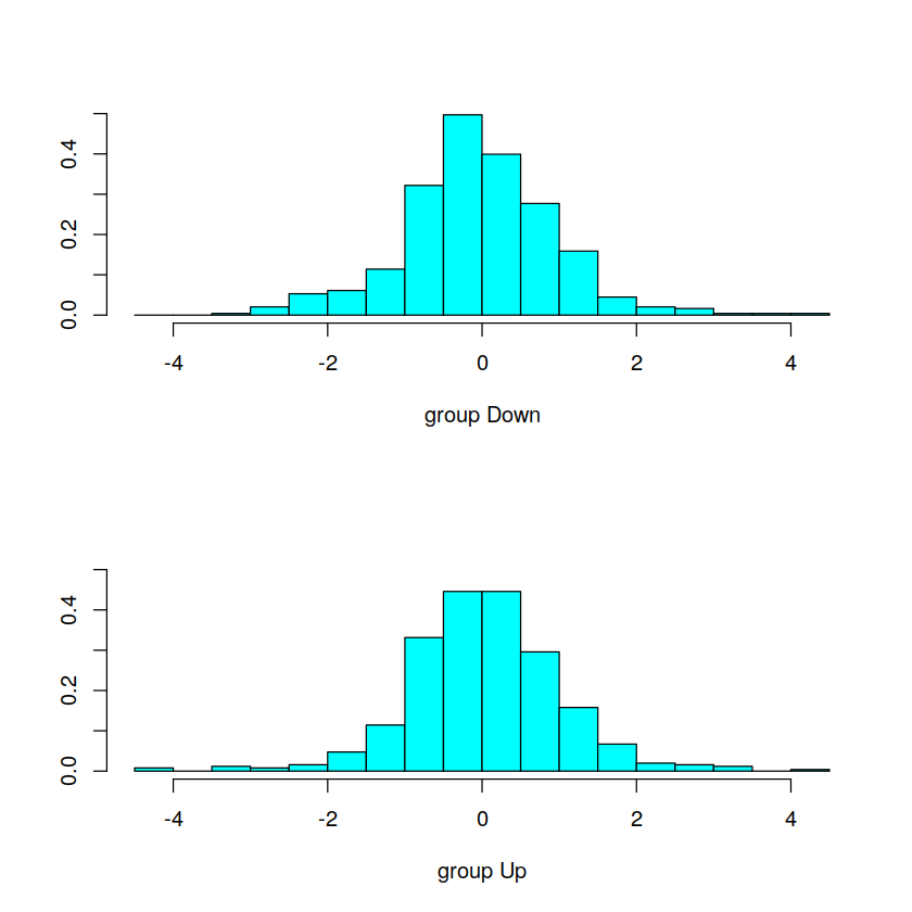
If $−0.642\times{\tt Lag1}−0.514\times{\tt Lag2}$ is large, then the LDA classifier will predict a market increase, and if it is small, then the LDA classifier will predict a market decline.

We can use the plot() function to produce plots of the linear discriminants, obtained by computing $−0.642\times{\tt Lag1}−0.514\times{\tt Lag2}$ for each of the training observations.

plot(model_LDA)

The predict() function returns a list with three elements. The first element, class, contains LDA’s predictions about the movement of the market. The second element, posterior, is a matrix whose $k^{th}$ column contains the posterior probability that the corresponding observation belongs to the $k^{th}$ class. Finally, x contains the linear discriminants, described earlier.

predictions_LDA = data.frame(predict(model_LDA, test))
names(predictions_LDA)

Let's check out the confusion matrix to see how this model is doing. We'll want to compare the predicted class (which we can find in the class column of the predictions_LDA data frame) to the true class.

predictions_LDA_2 = cbind(test, predictions_LDA)

predictions_LDA_2 %>%
  count(class, Direction)

predictions_LDA_2 %>%
  summarize(score = mean(class == Direction))

The LDA predictions are identical to the ones from our logistic model:

# Logistic model, for comparison
model_logistic = glm(Direction~Lag1+Lag2, data=train ,family=binomial)

logistic_probs = data.frame(probs = predict(model_logistic, test, type="response"))

predictions_logistic = logistic_probs %>%
  mutate(class = ifelse(probs>.5, "Up", "Down"))

predictions_logistic = cbind(test, predictions_logistic)

predictions_logistic %>%
  count(class, Direction)

predictions_logistic %>%
  summarize(score = mean(class == Direction))

4.6.4 Quadratic Discriminant Analysis¶

We will now fit a QDA model to the Smarket data. QDA is implemented in R using the qda() function, which is also part of the MASS library. The syntax is identical to that of lda().

model_QDA = qda(Direction~Lag1+Lag2, data = train)
model_QDA

Call:
qda(Direction ~ Lag1 + Lag2, data = train)

Prior probabilities of groups:
 Down    Up 
0.492 0.508 

Group means:
         Lag1     Lag2
Down  0.04279  0.03389
Up   -0.03955 -0.03133

The output contains the group means. But it does not contain the coefficients of the linear discriminants, because the QDA classifier involves a quadratic, rather than a linear, function of the predictors. The predict() function works in exactly the same fashion as for LDA.

predictions_QDA = data.frame(predict(model_QDA, test))

predictions_QDA = cbind(test, predictions_QDA)

predictions_QDA %>%
  count(class, Direction)

predictions_QDA %>%
  summarize(score = mean(class == Direction))

Interestingly, the QDA predictions are accurate almost 60% of the time, even though the 2005 data was not used to fit the model. This level of accuracy is quite impressive for stock market data, which is known to be quite hard to model accurately.

This suggests that the quadratic form assumed by QDA may capture the true relationship more accurately than the linear forms assumed by LDA and logistic regression. However, we recommend evaluating this method’s performance on a larger test set before betting that this approach will consistently beat the market!

A data.frame: 4 × 3
class	Direction	n
<fct>	<fct>	<int>
Down	Down	35
Down	Up	35
Up	Down	76
Up	Up	106

A data.frame: 1 × 1
score
<dbl>
0.5595

A data.frame: 4 × 3
class	Direction	n
<chr>	<fct>	<int>
Down	Down	35
Down	Up	35
Up	Down	76
Up	Up	106

A data.frame: 1 × 1
score
<dbl>
0.5595