Geovisualization with PySAL
Introduction
When the Python Spatial Analysis Library, PySAL, was originally planned, the intention was to focus on the computational aspects of exploratory spatial data analysis and spatial econometric methods, while relying on existing GIS packages and visualization libraries for visualization of computations. Indeed, we have partnered with esri and QGIS towards this end.
However, over time we have received many requests for supporting basic geovisualization within PySAL so that the step of having to interoperate with an external package can be avoided, thereby increasing the efficiency of the spatial analytical workflow.
In this notebook, we demonstrate several approaches towards a particular subset of geovisualization methods, namely choropleth maps. We start with an exploratory workflow introducing mapclassify and geopandas to create different choropleth classifications and maps for quick exploratory data analysis. We then introduce the geoviews package for interactive mapping in support of exploratory spatial data analysis.
PySAL Map Classifiers
import mapclassify
import geopandas as gpd
import matplotlib.pyplot as plt
import contextily as cx
shp_link = 'data/scag_region.gpkg'
gdf = gpd.read_file(shp_link)
gdf = gdf.to_crs(3857)
f, ax = plt.subplots(1, figsize=(12, 8))
gdf.plot(column='median_home_value', scheme='QUANTILES', ax=ax,
edgecolor='white', legend=True, linewidth=0.3)
ax.set_axis_off()
plt.show()
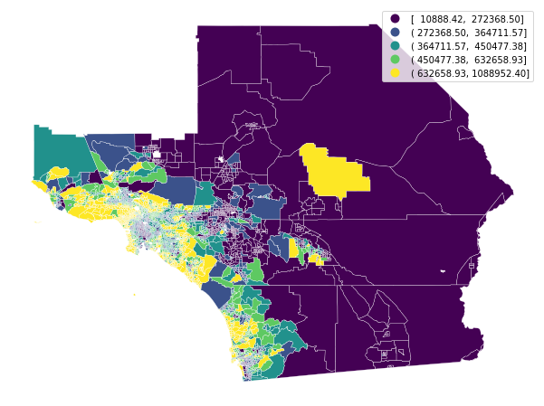
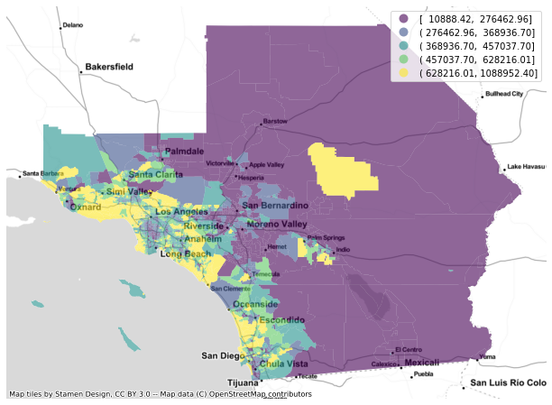
As a first cut, geopandas makes it very easy to plot a map quickly. If you know the area well, this may do fine for quick exploration. If you don't know a place extremely well (or you want to make a figure easy to understand for those who don't) it's often a good idea to add a basemap for context. We can do that easily using the contextily package
gdf.fillna(gdf.mean(), inplace = True)
f, ax = plt.subplots(1, figsize=(12, 8))
gdf.plot(column='median_home_value', scheme='QUANTILES', alpha=0.6, ax=ax, legend=True)
cx.add_basemap(ax, crs=gdf.crs.to_string(), source=cx.providers.Stamen.TonerLite)
ax.set_axis_off()
plt.show()

hv = gdf['median_home_value']
mapclassify.Quantiles(hv, k=5)
mapclassify.Quantiles(hv, k=10)
q10 = mapclassify.Quantiles(hv, k=10)
dir(q10)
q10.bins
q10.counts
fj10 = mapclassify.FisherJenks(hv, k=10)
fj10
fj10.adcm
q10.adcm
bins = [100000, 500000, 1000000, 1500000]
ud4 = mapclassify.UserDefined(hv, bins=bins)
ud4
GeoPandas: Choropleths
f, ax = plt.subplots(1, figsize=(12, 8))
gdf.plot(column='median_home_value', scheme='QUANTILES', ax=ax, alpha=0.6, legend=True)
cx.add_basemap(ax, crs=gdf.crs.to_string(), source=cx.providers.Stamen.TonerLite)
ax.set_axis_off()
plt.show()
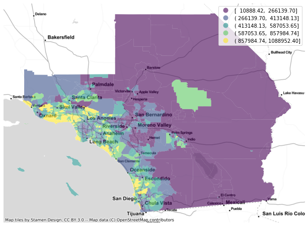
f, ax = plt.subplots(1, figsize=(12, 8))
gdf.plot(column='median_home_value', scheme='FisherJenks', ax=ax,
alpha=0.6, legend=True)
cx.add_basemap(ax, crs=gdf.crs.to_string(), source=cx.providers.Stamen.TonerLite)
ax.set_axis_off()
plt.show()
gdf.geoid
import numpy
counties = set([geoid[:5] for geoid in gdf.geoid])
counties
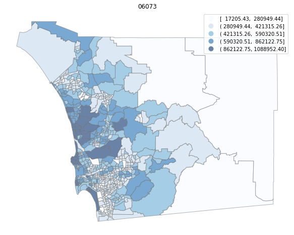
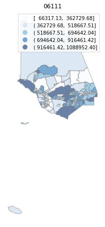
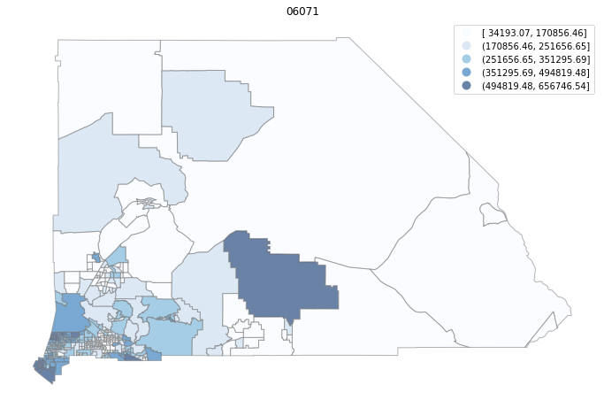
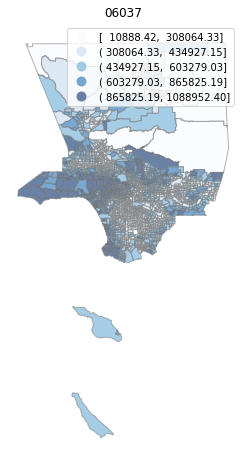
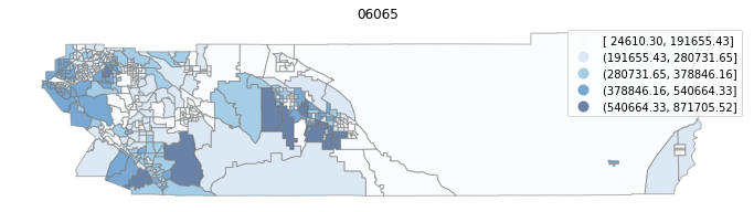
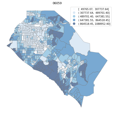
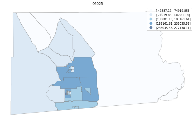
for county in counties:
cgdf = gdf[gdf['geoid'].str.match(f'^{county}')]
f, ax = plt.subplots(1, figsize=(12, 8))
cgdf.plot(column='median_home_value', scheme='FisherJenks', ax=ax,
edgecolor='grey', legend=True, cmap='Blues', alpha=0.6)
plt.title(county)
ax.set_axis_off()
plt.show()
Geoviews
import geoviews as gv
import geoviews.feature as gf
import xarray as xr
from cartopy import crs
import hvplot.pandas
import geopandas as gpd
cities = gpd.read_file(gpd.datasets.get_path('naturalearth_cities'))
cities.hvplot(global_extent=True, frame_height=450, tiles=True)
shp_link = 'data/scag_region.gpkg'
gdf = gpd.read_file(shp_link)
gdf.fillna(gdf.mean(), inplace = True)
%%time
gdf.hvplot()
gdf.hvplot(geo=True)
def choro(df, field, scheme='Quantiles', ncolors=5, cmap='Blues',
width=1000, height=700, tools=['hover']):
from holoviews.plotting.util import process_cmap
cl = getattr(mapclassify, scheme)
yb = cl(df[field], k=ncolors).yb
pcmap = process_cmap(cmap, ncolors=ncolors)
df[scheme] = yb
return gv.Polygons(df, vdims=[scheme, field]).opts(cmap=pcmap, width=width, height=height, tools=tools, line_width=0.1)
choro(gdf, 'median_home_value')
choro(gdf, 'median_home_value', ncolors=9, cmap='viridis')
(gv.tile_sources.CartoLight * choro(gdf, 'median_home_value', scheme='FisherJenks', ncolors=9, cmap='viridis'))
Create choropleth maps for each of the counties that use the FisherJenks classification for k=6 defined on the entire Southern California region.
# %load solutions/01.py

<span
xmlns:dct="http://purl.org/dc/terms/" property="dct:title">Geovisualization</span> by <a xmlns:cc="http://creativecommons.org/ns#"
href="http://sergerey.org" property="cc:attributionName"
rel="cc:attributionURL">Serge Rey</a> is licensed under a Creative
Commons Attribution-NonCommercial-ShareAlike 4.0 International License.