NMF Topic Models
Topic modelling aims to automatically discover the hidden thematic structure in a large corpus of text documents. One approach for topic modelling is to apply matrix factorisation methods, such as Non-negative Matrix Factorisation (NMF). In this notebook we look at how to apply NMF using the scikit-learn library in Python.
Applying NMF
First, let's load the TF-IDF normalised document-term matrix and list of terms that we stored earlier using Joblib:
import joblib
(A,terms,snippets) = joblib.load( "articles-tfidf.pkl" )
print( "Loaded %d X %d document-term matrix" % (A.shape[0], A.shape[1]) )
The key input parameter to NMF is the number of topics to generate k. For the moment, we will pre-specify a guessed value, for demonstration purposes.
k = 10
Another choice for NMF revolves around initialisation. Most commonly, NMF involves using random initialisation to populate the values in the factors W and H. Depending on the random seed that you use, you may get different results on the same dataset. Instead, using SVD-based initialisation provides more reliable results.
# create the model
from sklearn import decomposition
model = decomposition.NMF( init="nndsvd", n_components=k )
# apply the model and extract the two factor matrices
W = model.fit_transform( A )
H = model.components_
Examining the Output
NMF produces to factor matrices as its output: W and H.
The W factor contains the document membership weights relative to each of the k topics. Each row corresponds to a single document, and each column correspond to a topic.
W.shape
For instance, for the first document, we see that it is strongly associated with one topic. However, each document can be potentially associated with multiple topics to different degrees.
# round to 2 decimal places for display purposes
W[0,:].round(2)
The H factor contains the term weights relative to each of the k topics. In this case, each row corresponds to a topic, and each column corresponds to a unique term in the corpus vocabulary.
H.shape
For instance, for the term "brexit", we see that it is strongly associated with a single topic. Again, in some cases each term can be associated with multiple topics.
term_index = terms.index('brexit')
# round to 2 decimal places for display purposes
H[:,term_index].round(2)
Topic Descriptors
The top ranked terms from the H factor for each topic can give us an insight into the content of that topic. This is often called the topic descriptor. Let's define a function that extracts the descriptor for a specified topic:
import numpy as np
def get_descriptor( terms, H, topic_index, top ):
    # reverse sort the values to sort the indices
    top_indices = np.argsort( H[topic_index,:] )[::-1]
    # now get the terms corresponding to the top-ranked indices
    top_terms = []
    for term_index in top_indices[0:top]:
        top_terms.append( terms[term_index] )
    return top_terms
We can now get a descriptor for each topic using the top ranked terms (e.g. top 10):
descriptors = []
for topic_index in range(k):
    descriptors.append( get_descriptor( terms, H, topic_index, 10 ) )
    str_descriptor = ", ".join( descriptors[topic_index] )
    print("Topic %02d: %s" % ( topic_index+1, str_descriptor ) )
The rankings above do not show the strength of association for the different terms. We can represent the distribution of the weights for the top terms in a topic using a matplotlib horizontal bar chart.
%matplotlib inline
import numpy as np
import matplotlib
import matplotlib.pyplot as plt
plt.style.use("ggplot")
matplotlib.rcParams.update({"font.size": 14})
Define a function to create a bar chart for the specified topic, based on the H factor from the current NMF model:
def plot_top_term_weights( terms, H, topic_index, top ):
    # get the top terms and their weights
    top_indices = np.argsort( H[topic_index,:] )[::-1]
    top_terms = []
    top_weights = []
    for term_index in top_indices[0:top]:
        top_terms.append( terms[term_index] )
        top_weights.append( H[topic_index,term_index] )
    # note we reverse the ordering for the plot
    top_terms.reverse()
    top_weights.reverse()
    # create the plot
    fig = plt.figure(figsize=(13,8))
    # add the horizontal bar chart
    ypos = np.arange(top)
    ax = plt.barh(ypos, top_weights, align="center", color="green",tick_label=top_terms)
    plt.xlabel("Term Weight",fontsize=14)
    plt.tight_layout()
    plt.show()
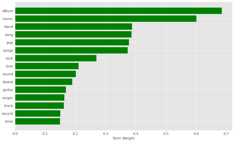
So for instance, for the 7th topic we can generate a plot with the top 15 terms using:
plot_top_term_weights( terms, H, 6, 15 )
Most Relevant Documents
We can also look at the snippets for the top-ranked documents for each topic. We'll define a function to produce this ranking also.
def get_top_snippets( all_snippets, W, topic_index, top ):
    # reverse sort the values to sort the indices
    top_indices = np.argsort( W[:,topic_index] )[::-1]
    # now get the snippets corresponding to the top-ranked indices
    top_snippets = []
    for doc_index in top_indices[0:top]:
        top_snippets.append( all_snippets[doc_index] )
    return top_snippets
For instance, for the first topic listed above, the top 10 documents are:
topic_snippets = get_top_snippets( snippets, W, 0, 10 )
for i, snippet in enumerate(topic_snippets):
    print("%02d. %s" % ( (i+1), snippet ) )
Similarly, for the second topic:
topic_snippets = get_top_snippets( snippets, W, 1, 10 )
for i, snippet in enumerate(topic_snippets):
    print("%02d. %s" % ( (i+1), snippet ) )
Exporting the Results
If we want to keep this topic model for later user, we can save it using joblib:
joblib.dump((W,H,terms,snippets), "articles-model-nmf-k%02d.pkl" % k)