2025-09-29

Apologies for the interruption in coverage; I have a good excuse, henceforth known as The Agent (of both the ‘defying the Principal’ variety and the fast-learning natural/artificial variety).

links

papers

McCartan and Kuriwaki revisit the ecological inference problem of estimating granular measurements (say, conditional means) when only aggregate quantities are observed. Clear statements of identification assumptions (Coarsening at Random is the magical fairydust in the literature analogous to Unconfoundedness) and encompassing exposition of the fragmented literature, representation as a linear functional which enables the use of automatic debiased machine learning methods and accompanying sensitivity analysis, etc.
Crippa and Fedchenko on the identification of ranking/reward models from pairwise comparisons data. Nice exposition of connections between Bradley-Terry-Luce and discrete choice models widespread in econometrics.
Van der Laan et al on a tractable approach to estimate Inverse Reinforcement Learning (IRL) models, which learn reward functions from observed offline behaviour [assumed to be generated by an expert/optimizing agent]. This last point should make it amply clear that this is identical to the problem of learning structural parameters in economic models [e.g. discrete choice models of static and dynamic varieties, estimating games, etc.]. Related: Chelsea Finn’s bootcamp slides

code, music

ssh-list is a good tui for managing ssh connections.
ivmodels looks like a well-designed and thorough package for IV and related methods (k-class, LIML).
Joel Grus’ very on-brand Clod - dspy is now so powerful that you can just leave it in charge of your computer until it tries to delete the french language pack rm -fr /.
Igorrr’s new album is fantastic. Eclectic Baroque glitch electronic metal with nods to Mick Gordon’s doom soundtracks and Hans Zimmer’s dune soundtracks.

self-promotion

arxivdiff lets you diff papers on arxiv by creating temp git repositories and visualizing latex source diffs in a web UI. I use it a lot.
Apropos of the top of this post, the Agent is healthy and growing at a frankly alarming clip. If we know each other IRL, feel free to ping me for photos; new parents love inflicting baby photos on others and turns out I’m no different.

Adversarial Estimation of Statistical Models

Notes from working through Kaji, Manresa, Pouliot, which was published a couple of years ago and has some interesting ideas. Despite the paper making heavy use of modern ML ideas, however, the replication code is in matlab and therefore unusable by anyone under 45.

The paper addresses a fundamental problem in structural econometrics: estimating parameters when the likelihood is intractable but simulation is feasible, e.g. in dynamic models that have multiple periods and forward-looking behaviour. The standard approach in this setting is Simulated Method of Moments (SMM), which is very brittle.

The Setup:

Real data: ${X_{i}}_{i = 1}^{n} \sim P_{0}$ (unknown distribution)
Model: ${P_{θ} : θ \in Θ}$ where we can simulate $X_{i, θ} = T_{θ} (X_{i})$ synthetic observations
If $P_{θ}$ is very different from $P_{0}$ , it is easy to distinguish between $X_{i}$ and $\tilde{X}_{i}$ . Conversely, they are very difficult to tell apart, $θ$ must be a good parameter value.

This is starting to look like the key idea motivating Generative Adversarial Networks (GANs), where a good data density $P (X ∣ Y)$ is arrived at through a game between a Generator and a Discriminator, where the former generates fake and the latter attempts to distinguish between real and fake data. The difference in emphasis between learning $θ$ vs a good $P (X ∣ Y)$ motivates the choice of distance [Jensen-Shannon suffices for our purposes here but in training GANs, Wasserstein distance is preferred because it handles partially overlapping supports between real and synthetic data much better than JS].

Key Insight: Use a binary classifier (discriminator) $D : X \to [0, 1]$ to assess whether $θ$ generates data similar to $P_{0}$ :

$D (x) \approx 1$ means x looks “real”
$D (x) \approx 0$ means x looks “simulated”
$D (x) \approx 0.5$ means x is indistinguishable

This can be formulated as a minimax objective

\hat{θ} = ar g θ \in Θ min D \in D_{n} max [\frac{1}{n} i = 1 \sum n lo g D (X_{i}) + \frac{1}{m} i = 1 \sum m lo g (1 - D (X_{i, θ}))]

The inner maximization trains D to distinguish real from simulated data (standard binary cross-entropy)
When $θ$ is wrong, $P_{θ} \neq = P_{0}$ , so a good discriminator achieves high accuracy (objective $\to$ 0)
When $θ$ is correct, $P_{θ} \approx P_{0}$ , so the best D can do is random guessing (objective $\to$ 2 log(1/2))
The outer minimization finds $θ$ where the discriminator is most confused

The oracle discriminator is $D_{θ} (x) = p_{θ} (x) / (p_{0} (x) + p_{θ} (x))$ . Under correct specification, $θ_{0}$ uniquely minimizes the population objective. With flexible discriminators (neural networks), the estimator can achieve parametric efficiency.

I implemented the basic approach for the toy examples in section 3 of the paper. I think this could generalize pretty reasonably, but as with GANs i think the theoretical elegance is far greater than the practical feasibility of solving adversarial problems.

import numpy as np
import matplotlib.pyplot as plt
from scipy.optimize import minimize
from scipy.stats import logistic, norm
from scipy.special import expit
from typing import Callable, Dict, Tuple, Optional
 
plt.rcParams["figure.figsize"] = (12, 4)
 
class AdversarialEstimator:
    """
    Adversarial estimation for simulation-based inference.
 
    Solves: θ̂ = argmin_θ max_D [E[log D(X)] + E[log(1-D(X_θ))]]
    """
 
    def __init__(
        self,
        simulator: Callable[[float, np.ndarray], np.ndarray],
        discriminator_fn: Callable[[np.ndarray, np.ndarray], np.ndarray],
        n_disc_params: int,
        disc_optimizer: str = "L-BFGS-B",
        disc_options: Optional[Dict] = None,
    ):
        """
        Args:
            simulator: Function (theta, shocks) -> simulated_data
            discriminator_fn: Function (x, params) -> probabilities
            n_disc_params: Number of discriminator parameters
            disc_optimizer: Scipy optimizer for discriminator training
            disc_options: Options dict for discriminator optimizer
        """
        self.simulator = simulator
        self.discriminator_fn = discriminator_fn
        self.n_disc_params = n_disc_params
        self.disc_optimizer = disc_optimizer
        self.disc_options = disc_options or {"maxiter": 100, "ftol": 1e-9}
 
    def train_discriminator(
        self,
        real_data: np.ndarray,
        sim_data: np.ndarray,
        eps: float = 1e-8,
    ) -> Tuple[np.ndarray, float]:
        """
        Train discriminator to distinguish real from simulated data.
 
        Maximizes: (1/n)Σ log D(Xi) + (1/m)Σ log(1-D(Xi,θ))
 
        Args:
            real_data: Real observations, shape (n,)
            sim_data: Simulated observations, shape (m,)
            eps: Small constant for numerical stability
 
        Returns:
            (optimal_params, objective_value)
        """
 
        def neg_objective(params):
            """Negative of discriminator objective for minimization."""
            D_real = self.discriminator_fn(real_data, params)
            D_sim = self.discriminator_fn(sim_data, params)
 
            obj = np.mean(np.log(D_real + eps)) + np.mean(np.log(1 - D_sim + eps))
            return -obj
 
        # discriminator parameter vector has variable length; can be sieve
        result = minimize(
            neg_objective,
            x0=np.zeros(self.n_disc_params),
            method=self.disc_optimizer,
            options=self.disc_options,
        )
 
        return result.x, -result.fun
 
    def objective(
        self, theta: float, real_data: np.ndarray, shocks: np.ndarray
    ) -> float:
        """
        Compute adversarial objective for given parameter.
 
        This is the inner maximization over discriminators.
 
        Args:
            theta: Parameter value
            real_data: Real observationsjensen
            shocks: Random shocks for simulation
 
        Returns:
            Objective value (more negative = better fit)
        """
        sim_data = self.simulator(theta, shocks)
        _, obj_value = self.train_discriminator(real_data, sim_data)
        return obj_value
 
    def estimate(
        self,
        real_data: np.ndarray,
        shocks: np.ndarray,
        theta_bounds: Tuple[float, float] = (-2.0, 2.0),
        n_grid: int = 80,
        refine_method: str = "L-BFGS-B",
        refine_options: Optional[Dict] = None,
        verbose: bool = True,
    ) -> Dict:
        """
        Estimate parameter via adversarial estimation.
 
        Args:
            real_data: Real observations, shape (n,)
            shocks: Random shocks for simulation, shape (m,)
            theta_bounds: Search bounds for theta
            n_grid: Number of grid points for initial search
            refine_method: Scipy optimizer for refinement
            refine_options: Options for refinement optimizer
            verbose: Print progress
 
        Returns:
            Dictionary with estimation results
        """
        if verbose:
            print("Computing objective surface...")
 
        # Grid search
        theta_grid = np.linspace(theta_bounds[0], theta_bounds[1], n_grid)
        objectives = []
 
        for i, theta in enumerate(theta_grid):
            if verbose and (i + 1) % 20 == 0:
                print(f"  Point {i + 1}/{n_grid}")
            obj = self.objective(theta, real_data, shocks)
            objectives.append(obj)
 
        objectives = np.array(objectives)
 
        # Find minimum (most confused discriminator)
        theta_init = theta_grid[np.argmin(objectives)]
 
        if verbose:
            print(f"\nRefining estimate starting from θ = {theta_init:.4f}")
 
        # Refinement
        refine_options = refine_options or {"maxiter": 50, "ftol": 1e-6}
 
        def obj_func(theta):
            return self.objective(theta[0], real_data, shocks)
 
        result = minimize(
            obj_func,
            x0=[theta_init],
            method=refine_method,
            bounds=[theta_bounds],
            options=refine_options,
        )
 
        if verbose:
            print(f"Estimated θ̂ = {result.x[0]:.4f}")
            print(f"Final objective = {result.fun:.4f}")
            print(f"Convergence: {result.success}")
 
        return {
            "theta_hat": result.x[0],
            "theta_grid": theta_grid,
            "objectives": objectives,
            "optimization_result": result,
            "converged": result.success,
        }

The adversarial estimator class is generic. The key methods are

train_discriminator: Inner maximization over discriminator parameters
objective: Compute objective for a given $θ$ (trains discriminator + evaluates)
estimate: Outer minimization over $θ$ (grid search + refinement)

Discriminator functions and simulators are passed in, like so

adv_est = AdversarialEstimator(
    simulator=logistic_simulator,
    discriminator_fn=logistic_location_discriminator,
    n_disc_params=2
)
results = adv_est.estimate(real_data, shocks)

Correctly-specified

First example in the paper (sec 3). API is general:

define discriminator (cross-entropy loss with a single parameter in the oracle case)
define simulator (considerably more complex for real models)
MLE for comparison

def logistic_location_discriminator(
    x: np.ndarray,
    params: np.ndarray,
) -> np.ndarray:
    """
    Oracle Discriminator for logistic location model.
    D_λ(x) = Λ(λ₀ - 2log(1+e^(-x)) + 2log(1+e^(-x+λ₁)))
 
    Args:
        x: Data points, shape (n,)
        params: [λ₀, λ₁]
 
    Returns:
        Discriminator probabilities, shape (n,)
    """
    lam0, lam1 = params
    term1 = lam0
    term2 = -2 * np.log(1 + np.exp(-x))
    term3 = 2 * np.log(1 + np.exp(-x + lam1))
    logit = term1 + term2 + term3
    return expit(logit)
 
 
def compute_mle_logistic(data: np.ndarray) -> Tuple[float, float]:
    """MLE for logistic location model (median)."""
    theta_mle = np.median(data)
    se = np.sqrt(np.pi**2 / (3 * len(data)))
    return theta_mle, se
 
 
def experiment_1_correctly_specified():
    """Experiment 1: Logistic location model (correctly specified)."""
    np.random.seed(42)
 
    n = 3000
    m = 3000
    true_theta = 4.0
 
    # Generate data
    real_data = logistic.rvs(loc=true_theta, scale=1.0, size=n)
    shocks = logistic.rvs(loc=0, scale=1.0, size=m)
 
    def T_logistic(theta: float, shocks: np.ndarray) -> np.ndarray:
        """Simulate from Logistic(θ, 1)."""
        return theta + shocks
 
    # MLE
    theta_mle, se_mle = compute_mle_logistic(real_data)
    print(f"\nMLE: θ̂ = {theta_mle:.4f}, SE = {se_mle:.4f}")
 
    # Adversarial estimation
    estimator = AdversarialEstimator(
        simulator=T_logistic,
        discriminator_fn=logistic_location_discriminator,
        n_disc_params=2,
    )
 
    results = estimator.estimate(real_data, shocks, theta_bounds=(2.0, 6.0))
    theta_adv = results["theta_hat"]
 
    # Plot
    fig, axes = plt.subplots(1, 2, figsize=(12, 4))
 
    ax = axes[0]
    ax.plot(results["theta_grid"], results["objectives"], "b-", linewidth=2)
    ax.axvline(
        true_theta,
        color="red",
        linestyle="--",
        linewidth=2,
        label=f"True θ = {true_theta}",
    )
    ax.axvline(
        theta_adv,
        color="green",
        linestyle="--",
        linewidth=2,
        label=f"θ̂_adv = {theta_adv:.3f}",
    )
    ax.axhline(
        2 * np.log(0.5),
        color="gray",
        linestyle=":",
        linewidth=2,
        label="Random guessing",
    )
    ax.set_xlabel("θ", fontsize=12)
    ax.set_ylabel("Objective value", fontsize=12)
    ax.set_title("Adversarial Objective Surface", fontsize=13)
    ax.legend()
    ax.grid(True, alpha=0.3)
 
    ax = axes[1]
    estimates = [theta_mle, theta_adv]
    errors = [abs(theta_mle - true_theta), abs(theta_adv - true_theta)]
    labels = ["MLE", "Adversarial"]
    colors = ["blue", "green"]
 
    bars = ax.bar(
        range(len(labels)),
        estimates,
        color=colors,
        alpha=0.6,
        edgecolor="black",
        linewidth=1.5,
    )
    ax.axhline(true_theta, color="red", linestyle="--", linewidth=2, label="True θ")
 
    for i, (bar, err) in enumerate(zip(bars, errors)):
        height = bar.get_height()
        ax.text(
            bar.get_x() + bar.get_width() / 2.0,
            height,
            f"error: {err:.4f}",
            ha="center",
            va="bottom",
            fontsize=9,
        )
 
    ax.set_xticks(range(len(labels)))
    ax.set_xticklabels(labels, fontsize=11)
    ax.set_ylabel("Estimated θ", fontsize=12)
    ax.set_title("Comparison of Estimators", fontsize=13)
    # ax.legend()
    ax.grid(True, alpha=0.3, axis="y")
 
    plt.tight_layout()
    plt.suptitle("Experiment 1: Correctly Specified Model", fontsize=16, y=1.02)
    plt.savefig("exp1_correctly_specified.png", dpi=150, bbox_inches="tight")
    plt.show()
 
 
# %%
experiment_1_correctly_specified()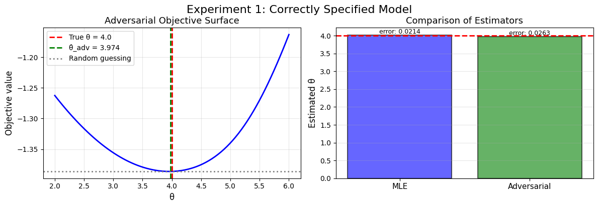

Misspecified (Normal/Logit)

second example in the paper. Data is still logistic, but we misspecify shocks to be normal.

def normal_logistic_discriminator(x: np.ndarray, params: np.ndarray) -> np.ndarray:
    """
    Discriminator for misspecified normal model.
    D_λ(x) = Λ(λ₀ + λ₁x + λ₂x² + λ₃log(1+e^(-x)))
 
    Args:
        x: Data points, shape (n,)
        params: [λ₀, λ₁, λ₂, λ₃]
 
    Returns:
        Discriminator probabilities, shape (n,)
    """
    features = np.stack([np.ones_like(x), x, x**2, np.log(1 + np.exp(-x))], axis=1)
    logit = features @ params
    return expit(logit)
 
 
def compute_quasi_mle_normal(data: np.ndarray) -> Tuple[float, float]:
    """Quasi-MLE: fit normal to data."""
    theta_qmle = np.mean(data)
    se = np.std(data, ddof=1) / np.sqrt(len(data))
    return theta_qmle, se
 
 
def experiment_2_misspecified():
    """Experiment 2: Misspecified normal model on logistic data."""
    np.random.seed(42)
 
    n = 600
    m = 600
    true_theta = 4.0
 
    # Real data: logistic, simulated shocks: normal (misspecified!)
    real_data = logistic.rvs(loc=true_theta, scale=1.0, size=n)
    shocks = norm.rvs(loc=0, scale=1.0, size=m)
 
    def T_normal(theta: float, shocks: np.ndarray) -> np.ndarray:
        """Simulate from N(θ, 1)."""
        return theta + shocks
 
    print(f"True data variance (logistic): {np.var(real_data):.2f}")
    print("Model variance (normal): 1.0")
    # Quasi-MLE
    theta_qmle, se_qmle = compute_quasi_mle_normal(real_data)
    print(f"Quasi-MLE: θ̂ = {theta_qmle:.4f}, SE = {se_qmle:.4f}")
 
    # Adversarial with misspecified model
    estimator = AdversarialEstimator(
        simulator=T_normal,  # Using normal!
        discriminator_fn=normal_logistic_discriminator,
        n_disc_params=4,
    )
 
    results = estimator.estimate(real_data, shocks, theta_bounds=(2.0, 6.0))
    theta_adv = results["theta_hat"]
 
    # Plot
    fig, axes = plt.subplots(1, 2, figsize=(12, 4))
 
    ax = axes[0]
    ax.plot(results["theta_grid"], results["objectives"], "b-", linewidth=2)
    ax.axvline(
        true_theta,
        color="red",
        linestyle="--",
        linewidth=2,
        label=f"True θ = {true_theta}",
    )
    ax.axvline(
        theta_adv,
        color="green",
        linestyle="--",
        linewidth=2,
        label=f"θ̂_adv = {theta_adv:.3f}",
    )
    ax.axhline(2 * np.log(0.5), color="gray", linestyle=":", linewidth=2)
    ax.set_xlabel("θ", fontsize=12)
    ax.set_ylabel("Objective value", fontsize=12)
    ax.set_title("Misspecified Model: Objective Surface", fontsize=13)
    ax.legend()
    ax.grid(True, alpha=0.3)
 
    ax = axes[1]
    estimates = [theta_qmle, theta_adv]
    errors = [abs(theta_qmle - true_theta), abs(theta_adv - true_theta)]
    labels = ["Quasi-MLE", "Adversarial"]
    colors = ["blue", "green"]
 
    bars = ax.bar(
        range(len(labels)),
        estimates,
        color=colors,
        alpha=0.6,
        edgecolor="black",
        linewidth=1.5,
    )
    ax.axhline(true_theta, color="red", linestyle="--", linewidth=2, label="True θ")
 
    for i, (bar, err) in enumerate(zip(bars, errors)):
        height = bar.get_height()
        ax.text(
            bar.get_x() + bar.get_width() / 2.0,
            height,
            f"error: {err:.4f}",
            ha="center",
            va="bottom",
            fontsize=9,
        )
 
    ax.set_xticks(range(len(labels)))
    ax.set_xticklabels(labels, fontsize=11)
    ax.set_ylabel("Estimated θ", fontsize=12)
    ax.set_title("Misspecified Model: Comparison", fontsize=13)
    # ax.legend()
    ax.grid(True, alpha=0.3, axis="y")
 
    plt.tight_layout()
    plt.suptitle("Experiment 2: Misspecified Model", fontsize=16, y=1.02)
    plt.savefig("exp2_misspecified.png", dpi=150, bbox_inches="tight")
    plt.show()
 
 
experiment_2_misspecified()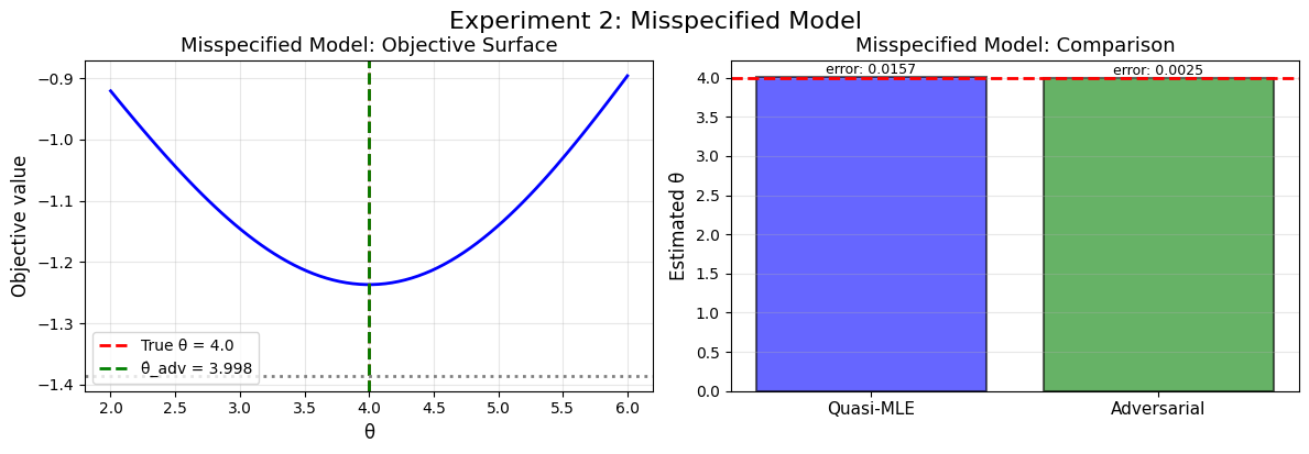

Somehow solving that weird minimax problem gives us good solutions in both cases!

Lalgorithms

Explorer