Naive Binning Is Fishy: Difference-in-Differences for Event Data

Abstract

Many empirical applications observe outcomes as event logs: transactions, calls for service, incidents, clicks, visits, or other timestamped arrivals. The usual difference-in-differences workflow bins these events into daily, weekly, or monthly counts and then estimates a linear two-way fixed-effects regression. The choice of time bin is inseparable from the scale on which the identifying restriction is imposed. For event data, a useful baseline model is a counting process with untreated intensities that factor into unit and calendar-time components. Under a proportional treatment effect on the intensity, the causal estimand is a rate ratio. A log rate-ratio difference-in-differences estimator and a Poisson fixed-effects estimator recover this object under multiplicative parallel trends. Linear fixed effects on binned counts instead impose additive parallel trends on the count scale; in general it estimates an additive rate or count contrast, not the log rate ratio. Changing the bin width cannot repair this scale mismatch and, for raw counts, mechanically changes the magnitude of the OLS coefficient. The analysis connects this point to Poisson pseudo-maximum likelihood in econometrics and to recurrent-event methods in biostatistics, and gives practical recommendations for event-log DiD designs.

Introduction

Event logs are now a common form of economic data. A platform records user actions; a city records calls for service; a hospital records admissions and readmissions; a firm records transactions; a website records visits. In all of these examples the primitive object is not a scalar outcome observed once per period but a timestamped point process. Applied work usually converts that process into a panel by choosing a calendar interval and counting events in each cell. The resulting outcome is then often analyzed with the same linear two-way fixed-effects tools used for continuous panel outcomes.

The conversion from event times to panel counts changes more than the sampling frequency. It also fixes the scale of the identifying restriction. When untreated event intensities follow multiplicative parallel trends, differences in baseline event rates across units are proportional rather than additive. If treatment has a proportional effect on the event intensity, the corresponding treatment effect is a log rate ratio. Poisson pseudo-maximum likelihood and a simple log rate-ratio DiD estimator are built for this scale. Linear regressions on binned counts are not.

The argument has four steps. First, a potential-outcome framework for counting processes leads directly to rate-ratio estimands for event data. Second, under untreated multiplicative parallel trends, a four-cell log rate-ratio estimator identifies the proportional treatment effect even when treated units have different baseline rates. Third, Poisson fixed effects consistently estimate the same log rate ratio when the binned conditional mean is exponential in unit, time, and treatment effects. The claim is quasi-likelihood: the conditional distribution need not literally be Poisson. Fourth, OLS on counts answers a different question. It can be a reasonable estimator of an additive count effect if additive parallel trends on counts is the target assumption, but it should not be interpreted as a percent lift or log rate ratio merely because the original data are finely binned.

Before binning event data, researchers should state whether the estimand is an additive change in expected counts, an additive change in rates, or a multiplicative change in rates. For most “lift” questions, the estimand is multiplicative. In those cases log rate-ratio DiD or Poisson/PPML fixed effects are the appropriate estimators, with exposure handled explicitly and with bins chosen so treatment status is not ambiguous within a cell.

Figure 1 gives the basic two-period logic. The treated group has a higher baseline event intensity than the control group, both groups experience a common inhomogeneous time pattern, and treatment raises the treated group’s post-$T_0$ intensity by 5 percent. The vertical gray lines are possible bins. The four numbers in the DiD contrasts are group-period average event rates: $0.50$ for control pre, $0.60$ for control post, $1.00$ for treated pre, and $1.26=1.00\times 1.20\times 1.05$ for treated post. With unit-width bins these are expected counts per bin; more generally they are expected counts divided by exposure. The log rate-ratio DiD recovers the 5 percent treatment effect because it compares proportional changes in rates, not differences in raw counts. The vanilla levels DiD is also well defined, but it reports $0.16$ rate units; normalized by the control pre-period mean, this is $0.16/0.50=32$ percent, far from the true 5 percent proportional lift.

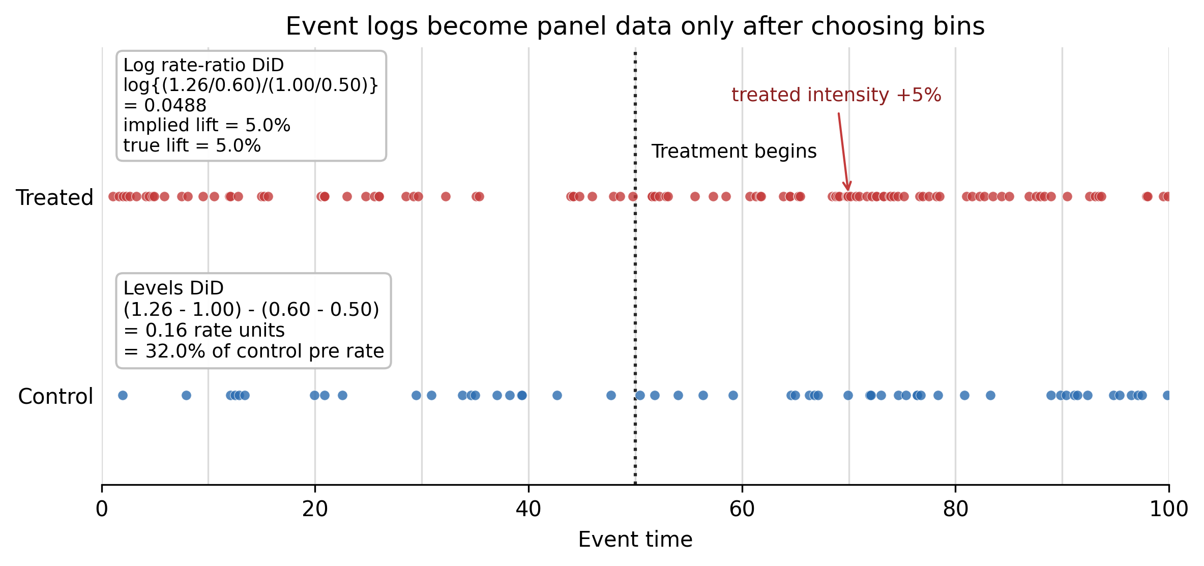
Figure 1. Event-time view of a two-period rate-ratio DiD. Dots are event times for treated and control groups. Gray lines show possible time bins; the dotted line marks treatment. The four numbers in the contrasts are group-period average event rates. The two-period log rate-ratio DiD equals the true 5 percent proportional effect; the levels DiD reports a different additive rate contrast, equal to 32 percent when normalized by the control pre-period rate.

Related Literature

The econometric foundation for this work is the pseudo-maximum likelihood literature. Poisson pseudo-likelihood can deliver consistent and asymptotically normal estimators under conditional-mean restrictions even when the full distribution is misspecified (Gourieroux, Monfort, and Trognon 1984a,b). Panel count models entered applied econometrics early in the patents and R&D literature (Hausman, Hall, and Griliches 1984). Fixed-effects Poisson estimators have useful robustness properties in multiplicative panel models when the conditional mean is correctly specified (Wooldridge 1999). The same logic became central in the trade literature: when the conditional mean is multiplicative and heteroskedasticity is present, log-linear OLS is generally not estimating the desired conditional-mean parameter (Santos Silva and Tenreyro 2006). Modern algorithms make Poisson models with high-dimensional fixed effects practical at large scale (Correia, Guimaraes, and Zylkin 2020). Recent nonlinear DiD work also develops exponential conditional-mean models for panel data (Wooldridge 2023). For timestamped event logs, the same conditional-mean logic applies after binning: exposure length and treatment timing determine the mean structure that PPML estimates.

The biostatistics and event-history literatures provide the stochastic-process language for the primitive outcome. The Cox model has a counting-process formulation, and there is a mature monograph literature on statistical models based on counting processes (Andersen and Gill 1982; Andersen et al. 1993). Recurrent-event methods are well developed (Cook and Lawless 2007), including semiparametric regression for recurrent-event mean and rate functions without requiring a Poisson process assumption (Lin et al. 2000). Competing risks and semicompeting risks have their own estimands, including cause-specific hazards, cumulative incidence functions, and subdistribution hazards; the subdistribution hazard model is the standard example (Fine and Gray 1999). Recent causal work explicitly formulates recurrent-event and competing-event estimands with potential outcomes and counting-process limits; Janvin et al. (2024) is closely related in its use of potential outcomes for recurrent event processes. Much of the causal recurrent-event literature identifies effects under observed covariate adjustment, sequential exchangeability, or structural hazard and mean-model restrictions. The DiD setting considered here instead allows treatment status to be related to time-invariant latent baseline intensity, provided untreated intensities satisfy a multiplicative parallel-trends restriction.

Relative to these literatures, the contribution is not a new event-history estimand or a new Poisson estimator. Familiar rate and mean-function estimands can be linked directly to DiD practice with timestamped event logs. The identifying restriction is a DiD restriction on untreated potential intensities: time-invariant baseline rate differences may be arbitrarily related to treatment status, but they enter multiplicatively and are removed by a rate-ratio contrast or by fixed effects in an exponential conditional mean. That link clarifies the role of temporal aggregation and explains why OLS on binned counts can fail when researchers intend to estimate a percent effect.

Counting-Process Setup

There are units $i=1,\dots ,n$ observed over a fixed horizon $[0,T]$. For unit $i$, $N_i(s,t]$ denotes the number of events in $(s,t]$, and $N_i(t)=N_i(0,t]$. In the main two-period design, some units are treated beginning at $T_0$ and others are never treated. Let $G_i\in \{0,1\}$ denote membership in the treated group and let $D_i(t)=G_{i}1\{t\ge T_0\}$.

For treatment regime $a\in \{0,1\}$, let $N_i^a(t)$ be the potential counting process and let ${\lambda }_i^a(t)$ be its predictable intensity. The compensator is

$${\Lambda }_i^a(t)={\int }_0^t{\lambda }_i^a(s)ds,$$

so that $N_i^a(t)-{\Lambda }_i^a(t)$ is a martingale under the usual event-history regularity conditions. The observed process satisfies consistency:

$$N_i(t)=N_i^{D_i(\cdot )}(t).$$

The post-treatment causal estimand is the proportional effect on expected event arrivals among the treated group:

$${\psi }_{\mathrm{ATT}}=\frac{\mathbb{E}\left[{\int }_{T_0}^T{\lambda }_i^1(t)dt\mid G_i=1\right]}{\mathbb{E}\left[{\int }_{T_0}^T{\lambda }_i^0(t)dt\mid G_i=1\right]},{\tau }_{\mathrm{ATT}}=\log {\psi }_{\mathrm{ATT}}.$$

The parameter is a causal rate ratio for cumulative event arrivals over a specified post-treatment window. If treatment has a constant proportional effect on the intensity, then ${\tau }_{\mathrm{ATT}}$ equals that log intensity ratio.

The target is a marginal rate ratio over a window, not a hazard ratio conditional on survival or on the full event history. For recurring events without terminal competing events, this is close to the marginal mean/rate function estimands used in recurrent-event analysis. If terminal or competing events are present, the estimand must be modified because time at risk is itself affected by treatment. That case requires the recurrent-event and competing-risk estimands studied in the biostatistics literature.

Identification in a Two-Period Design

Let $I_0=[0,T_0)$ and $I_1=[T_0,T]$. Write

$${\mu }_{gp}^a=\frac{1}{|I_p|}\mathbb{E}\left[N_i^a(I_p)\mid G_i=g\right],g,p\in \{0,1\}.$$

The identifying restriction is multiplicative parallel trends for untreated rates. There exist group-specific baseline factors $A_g>0$ and period-specific rate factors $B_p>0$ such that

$${\mu }_{gp}^0=A_g{B}_p.$$

This condition allows treated and control units to have different baseline event rates. It restricts the untreated evolution of rates to be proportional across groups.

The treatment effect restriction is proportionality in the treated post period:

$${\mu }_{11}^1=e^{\tau }{\mu }_{11}^0.$$

Together, these assumptions imply

$$\log \left(\frac{{\mu }_{11}/{\mu }_{01}}{{\mu }_{10}/{\mu }_{00}}\right)=\tau ,$$

where ${\mu }_{gp}$ denotes the observed group-period rate. The corresponding sample estimator is

$${\hat{\tau }}_{\mathrm{RR}}=\log \left(\frac{{\hat{\mu }}_{11}/{\hat{\mu }}_{01}}{{\hat{\mu }}_{10}/{\hat{\mu }}_{00}}\right),$$

with ${\hat{\mu }}_{gp}$ equal to total events divided by total exposure in cell $(g,p)$.

The same contrast obtains from a saturated Poisson model for the four cell totals with log exposure as an offset. The identifying assumption concerns expected rates: untreated expected rates are separable in group and period, and treatment multiplies the treated post rate.

Temporal Aggregation and Binned Counts

Applied researchers rarely estimate from the raw event times. They choose a partition $\mathcal{B}=\{B_1,\dots ,B_K\}$ of $[0,T]$ and construct

$$Y_{ik}=N_i(B_k).$$

Let $h_k=|B_k|$ denote exposure in bin $k$. If the untreated intensity has the form

$${\lambda }_i^0(t)=\exp ({\alpha }_i)g(t),$$

and treatment is constant within bin $B_k$, then

$$\mathbb{E}[Y_{ik}\mid {\alpha }_i,D_{ik}]=\exp ({\alpha }_i+\tau D_{ik}){\int }_{B_k}g(t)dt.$$

Equivalently,

$$\mathbb{E}[Y_{ik}\mid {\alpha }_i,D_{ik}]=\exp ({\alpha }_i+{\eta }_k+\tau D_{ik}),{\eta }_k=\log {\int }_{B_k}g(t)dt.$$

Therefore a Poisson fixed-effects regression with unit and bin effects is correctly specified at the level of the conditional mean, even if the baseline intensity varies within the bin. The bin fixed effect absorbs the integrated baseline intensity.

This exact representation requires treatment status to be constant within the bin. If a bin straddles a treatment adoption time, then the exact mean is

$$\mathbb{E}[Y_{ik}\mid {\alpha }_i]=\exp ({\alpha }_i)\left[{\int }_{B_k\cap \{D_i(t)=0\}}g(t)dt+e^{\tau }{\int }_{B_k\cap \{D_i(t)=1\}}g(t)dt\right],$$

which is generally not equal to $\exp ({\alpha }_i+{\eta }_k+\tau W_{ik})$ for a fractional exposure variable $W_{ik}$. Event-log applications should therefore split bins at treatment adoption times or include separate treated and untreated exposure components when treatment changes inside a bin.

The Poisson estimator solves the sample analogue of the conditional-mean moment condition

$$\mathbb{E}\left[Y_{ik}-\exp ({\alpha }_i+{\eta }_k+\tau D_{ik})\mid {\alpha }_i,{\eta }_k,D_{ik}\right]=0.$$

Interpreted this way, the estimator is PPML/QMLE. It does not require equidispersion, independent event arrivals, or a literal Poisson process, provided the conditional mean is correct and inference accounts for clustering or serial dependence.

What Linear Fixed Effects Estimates

OLS on binned counts imposes an additive conditional mean:

$$\mathbb{E}[Y_{ik}\mid {\alpha }_i,{\eta }_k,D_{ik}]=a_i+b_k+\delta D_{ik}.$$

The linear specification corresponds to additive parallel trends in counts, not multiplicative parallel trends in rates. Except in degenerate cases, additive and multiplicative parallel trends cannot both be true at the same time.

The distinction is visible in the two-by-two population coefficient. With equal exposure within period and untreated means ${\mu }_{gp}^0=A_g{B}_p$, the saturated linear DiD contrast is

$${\delta }_{\mathrm{OLS}}={\mu }_{11}-{\mu }_{10}-{\mu }_{01}+{\mu }_{00}=A_1(e^{\tau }{B}_1-B_0)-A_0(B_1-B_0).$$

If $\tau =0$, this equals $(A_1-A_0)(B_1-B_0)$, which is generally nonzero whenever treated and control units have different baseline rates and the common rate factor changes over time. If $B_1=B_0$, then

$${\delta }_{\mathrm{OLS}}=A_1{B}_1(e^{\tau }-1),$$

an additive rate or count effect for the treated group, not the log rate ratio $\tau$.

As bins shrink, a raw count coefficient changes with the exposure length of the bin. If counts are divided by exposure, the limiting object is an additive rate contrast. Neither object is a log rate ratio unless additional approximations are imposed. OLS can be appropriate for an additive count estimand. Without a model or transformation targeting a multiplicative estimand, it is not a percent-effect estimator.

Simulation Evidence

The simulation design varies treatment assignment while holding fixed a multiplicative event-rate data-generating process. Each replication has $n=100$ units observed over $T=50$ periods, with treatment beginning at $T_0=20$ for treated units. Unit heterogeneity is ${\alpha }_i\sim N(0,0.5^2)$ and the auxiliary covariate is $U_i\sim \mathrm{Uniform}(0,1)$. Conditional on these quantities, events are generated by an inhomogeneous Poisson process with intensity

$${\lambda }_i(t)=\exp \{{\alpha }_i+{\beta }_U{U}_i+\tau D_i(t)+\gamma (t)\},\gamma (t)=0.3\sin (2\pi t/7),$$

with a true log rate ratio $\tau =0.5$. The calendar component $\gamma (t)$ makes the process inhomogeneous but common across units.

There are three assignment designs. In the first, exactly half the units are treated at random and ${\beta }_U=0$. In the second, treatment depends on the unit fixed effect:

$$\mathbf{Pr}(G_i=1\mid {\alpha }_i)=\frac{\exp ({\alpha }_i)}{1+\exp ({\alpha }_i)},{\beta }_U=0.$$

This creates large baseline rate differences between treated and control units, but those differences are time invariant and therefore compatible with multiplicative parallel trends. In the third, treatment depends on an unobserved covariate:

$$\mathbf{Pr}(G_i=1\mid U_i)=\frac{\exp \{2(U_i-0.5)\}}{1+\exp \{2(U_i-0.5)\}},{\beta }_U=\mathrm{0.5.}$$

Here $U_i$ affects both treatment and the baseline event rate, but it is time invariant and enters the intensity multiplicatively, so the maintained DiD restriction is still satisfied.

The estimators are a four-cell log rate-ratio DiD estimator, Poisson fixed effects with fine and coarse bins, and linear fixed effects on raw counts with fine and coarse bins. Because the OLS coefficient is an additive count contrast rather than a log rate ratio, Figure 2 plots the linear estimates on their own scale.

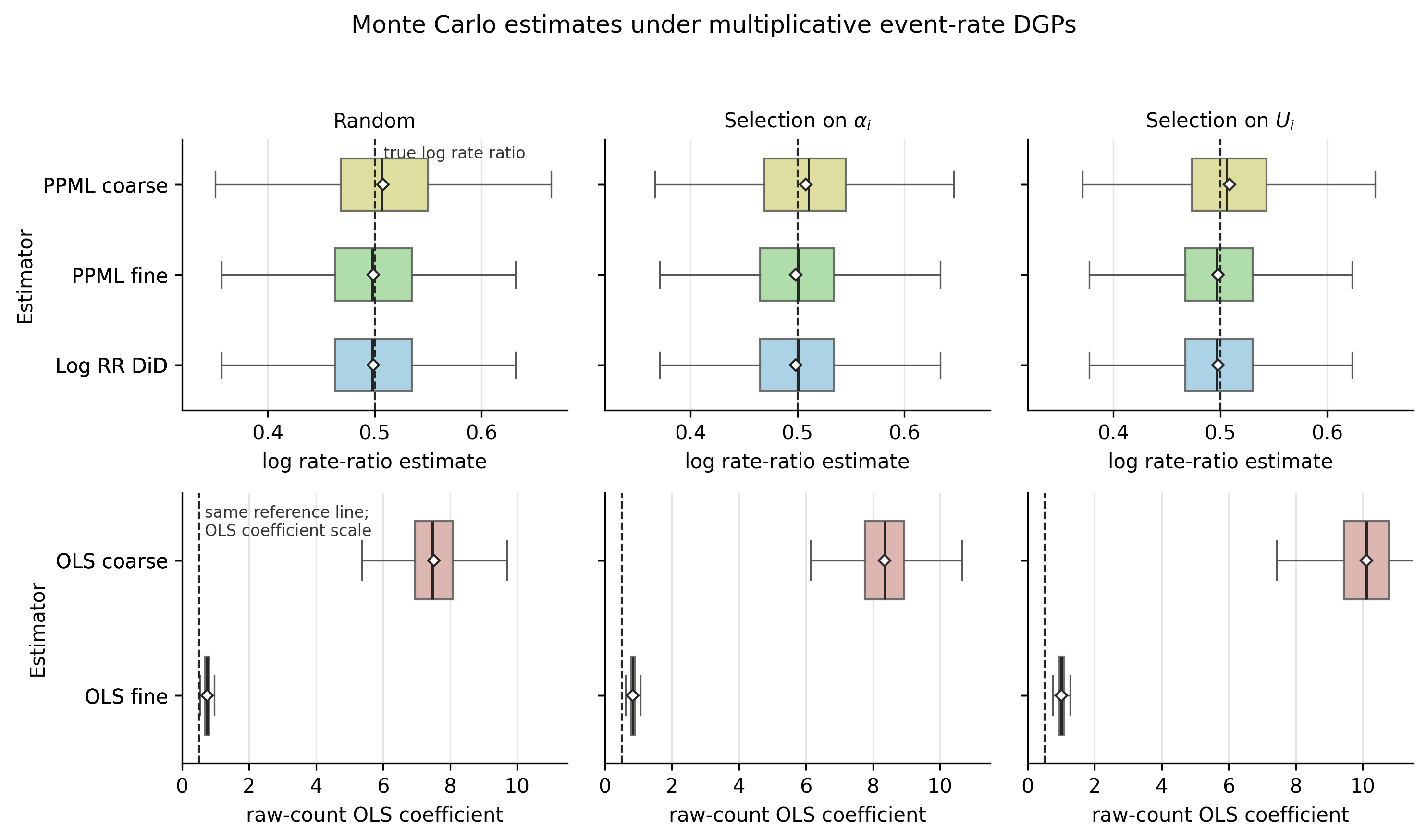
Figure 2. Monte Carlo estimates under three assignment designs. The top row shows estimators whose target is the log rate ratio. The dashed vertical line is the true value $\tau =0.5$. The bottom row shows OLS fixed-effect coefficients on raw binned counts; these are additive count effects, not log rate ratios.

Across all three assignment designs, the four-cell log rate-ratio DiD and the fine-bin Poisson fixed-effects estimator are centered at approximately $0.5$. The coarse-bin Poisson estimator is also close, with small deviations caused by coarse bins that can average over changes in treatment exposure or calendar intensity. Selection on ${\alpha }_i$ and selection on $U_i$ do not move these estimators because both variables shift baseline rates rather than untreated rate growth.

The OLS coefficients are on the raw-count scale. The fine-bin OLS coefficient is an additive count effect per fine interval, and the coarse-bin OLS coefficient is much larger because the outcome is a count over a longer exposure interval. Interpreting either coefficient as a log rate ratio would conflate additive and multiplicative estimands. The design would need additive parallel trends in expected counts, rather than multiplicative parallel trends in event rates, for those coefficients to be the primary causal object.

Event-Log Metrics and xAU Outcomes

Many applications do not use raw event counts. They first transform events into active-user metrics, such as DAU, WAU, or MAU:

$$\mathrm{xAU}(B_k)=\sum _{i}1\{N_i(B_k)>0\}.$$

Active-user outcomes are another form of temporal aggregation. For a Poisson process with integrated intensity ${\Lambda }_i(B_k)$,

$$\mathbb{P}\{N_i(B_k)>0\}=1-\exp \{-{\Lambda }_i(B_k)\}.$$

If treatment multiplies the underlying event intensity by $e^{\tau }$, the induced effect on the active-user probability is

$$\frac{1-\exp \{-e^{\tau }{\Lambda }_i^0(B_k)\}}{1-\exp \{-{\Lambda }_i^0(B_k)\}},$$

which depends on the baseline integrated intensity and the window length. For rare events or very short windows this ratio is close to $e^{\tau }$. For common events or long windows it is attenuated toward one because the active indicator saturates.

Thus xAU effects are not merely rate-ratio effects with a different label. The window length is part of the estimand. Researchers analyzing active-user outcomes should state whether the target is the effect on event intensity, the effect on the probability of at least one event in a specified window, or the effect on the count of active units.

Practical Recommendations

For event-log DiD designs, the following workflow is defensible.

1. State the primitive outcome: raw event counts, rates per exposure, active-user indicators, first-event times, or recurrent events with terminal competing events.

2. State the causal scale: additive count difference, additive rate difference, log rate ratio, risk difference, or risk ratio.

3. If the target is a log rate ratio, use a log rate-ratio DiD estimator in the two-by-two case or a Poisson/PPML fixed-effects estimator in richer panel designs.

4. Include exposure explicitly. With unequal bin widths or varying time at risk, include log exposure as an offset or use bin fixed effects that absorb the relevant integrated exposure only when appropriate.

5. Split bins at treatment adoption times. Fractional treatment indicators inside nonlinear mean models are approximations unless the exposure model is written exactly.

6. Use robust or clustered inference. The Poisson likelihood is a convenient estimating criterion, not a maintained assumption that events are independent and equidispersed.

7. Treat OLS on counts as estimating an additive count or rate contrast. Do not interpret the coefficient as a percent effect unless the model has been transformed or rescaled to target that object.

Conclusion

Event-log data make the time scale of analysis explicit. The choice of bin width is not a harmless preprocessing step because it interacts with the scale of the identifying restriction and the scale of the estimand. Under multiplicative parallel trends for untreated event rates, the natural DiD estimand is a log rate ratio. Poisson fixed effects and the four-cell log rate-ratio estimator target that object. Linear fixed effects on binned counts generally target an additive count or rate contrast instead. The resulting discrepancy is not fixed by making bins smaller; it is a mismatch between the causal question and the regression mean function.

References

• Andersen, Per K., Ornulf Borgan, Richard D. Gill, and Niels Keiding. 1993. Statistical Models Based on Counting Processes. Springer.
• Andersen, Per K., and Richard D. Gill. 1982. “Cox’s Regression Model for Counting Processes: A Large Sample Study.” The Annals of Statistics 10(4): 1100-1120.
• Cook, Richard J., and Jerald F. Lawless. 2007. The Statistical Analysis of Recurrent Events. Springer.
• Correia, Sergio, Paulo Guimaraes, and Thomas Zylkin. 2020. “Fast Poisson Estimation with High-Dimensional Fixed Effects.” The Stata Journal 20(1): 95-115.
• Fine, Jason P., and Robert J. Gray. 1999. “A Proportional Hazards Model for the Subdistribution of a Competing Risk.” Journal of the American Statistical Association 94(446): 496-509.
• Gourieroux, Christian, Alain Monfort, and Alain Trognon. 1984a. “Pseudo Maximum Likelihood Methods: Applications to Poisson Models.” Econometrica 52(3): 701-720.
• Gourieroux, Christian, Alain Monfort, and Alain Trognon. 1984b. “Pseudo Maximum Likelihood Methods: Theory.” Econometrica 52(3): 681-700.
• Hausman, Jerry A., Bronwyn H. Hall, and Zvi Griliches. 1984. “Econometric Models for Count Data with an Application to the Patents-R&D Relationship.” Econometrica 52(4): 909-938.
• Janvin, Matias, Jessica G. Young, Pal C. Ryalen, and Mats J. Stensrud. 2024. “Causal Inference with Recurrent and Competing Events.” Lifetime Data Analysis 30: 59-118.
• Lin, D. Y., L. J. Wei, I. Yang, and Z. Ying. 2000. “Semiparametric Regression for the Mean and Rate Functions of Recurrent Events.” Journal of the Royal Statistical Society: Series B 62(4): 711-730.
• Santos Silva, J. M. C., and Silvana Tenreyro. 2006. “The Log of Gravity.” The Review of Economics and Statistics 88(4): 641-658.
• Wooldridge, Jeffrey M. 1999. “Distribution-Free Estimation of Some Nonlinear Panel Data Models.” Journal of Econometrics 90(1): 77-97.
• Wooldridge, Jeffrey M. 2023. “Simple Approaches to Nonlinear Difference-in-Differences with Panel Data.” The Econometrics Journal 26(3): C31-C66.