Half a dozen ways to turn LLMs into a discrete choice model

github repo

Abstract

Can an autoregressive language model serve as a probability estimator for a finite choice problem with text-rich covariates? We analyze several empirical approaches including vocabulary normalization, frozen LLM scoring, in-context conditioning, quantized low-rank adaptation, and validation-estimated calibration to standard tabular methods. The empirical application predicts the most-played title among five games in a Steam user’s library using non-candidate play histories, reviews, and product metadata. On a held-out test sample of 1,000 choice sets, a naive popularity rule reaches 0.404 accuracy, conditional logit reaches 0.461, while naively renormalizing Qwen3.5-4B label likelihoods reach just 0.286 accuracy. A specification combining a 3.15-million-parameter QLoRA adapter, the training-format instruction, and five in-context examples reaches 0.462; affine calibration raises accuracy to 0.480.

Introduction

Discrete-choice models map information about decision makers and alternatives into probabilities on a finite set. In a conventional random-utility model, the analyst writes a systematic index and derives a probability kernel from assumptions on the stochastic component (McFadden 1974; Train 2009). Modern empirical settings also contain semi-structured and mixed data including product characteristics, histories, descriptions, tags, reviews, and multi-modal information that are awkward to compress into a prespecified index. A language model offers a rich nonlinear map of those inputs, but its native output is a distribution over text rather than economic alternatives.

A simple approach is to simply normalize logits. Given a fixed context, the network’s final layer produces one logit for every vocabulary token. A vocabulary softmax converts those logits into next-token probabilities. For a multi-token answer, a deterministic forward pass supplies the probability of each successive token conditional on the fixed preceding tokens; summing their log probabilities gives the likelihood of the entire answer string. No answer need be sampled. If $S_j$ is the answer string assigned to alternative $j$, its log likelihood can serve as an alternative-specific index,

$$L_{ij}=\log p_{\theta }(S_j\mid q_i),$$

and the analyst can condition the admissible strings on the observed set,

$${\pi }_{ij}=\frac{\exp (L_{ij})}{{\sum }_{k\in C_i}\exp (L_{ik})}.$$

This second normalization is what creates a probability vector on $C_i$. It addresses the same candidate-string and surface-form problem studied in language-model multiple-choice scoring (Holtzman et al. 2021). It is nevertheless a normalization, not a behavioral derivation: no extreme-value disturbance has been estimated or assumed merely because the final formula resembles logit.

We compare four ways to construct or modify this index. Frozen scoring uses only pretrained parameters. In-context learning (ICL) conditions the model on labeled examples without changing its weights. Quantized low-rank adaptation (QLoRA) estimates a persistent low-rank correction to selected attention matrices. An affine calibration model estimates a common scale and position-specific constants from validation probabilities. We also evaluate whether activation steering, which adds a supervised direction to an internal representation without updating network weights, can supply a lower-dimensional alternative to QLoRA. Local inference uses a four-bit Qwen3.5-4B model on a 12 GB GPU; the numerical formats and estimation criteria are defined below.

The empirical application is a five-alternative prediction problem. Each observation contains five games in a Steam user’s library, and the outcome is the title with the greatest recorded lifetime playtime. Candidate playtime is withheld; predictors include non-candidate play and review histories, user aggregates, and candidate metadata. The setting supplies observed behavioral labels and rich text while keeping the prediction target and leakage controls transparent.

The main empirical benchmark is a conditional logit that imposes common attribute coefficients across randomly ordered positions. It reaches 0.461 accuracy and negative log likelihood 1.335, compared with 0.416 and 1.450 for a pooled position-specific classifier. Frozen label likelihoods reach only 0.286 accuracy. The jointly adapted Qwen specification reaches 0.462, and affine calibration raises it to 0.480 with negative log likelihood 1.345.

The paper sits between four literatures. Neural choice models already replace or augment analyst-written utility with learned representations (Sifringer, Lurkin, and Alahi 2020; Han et al. 2022; van Cranenburgh et al. 2022). Work in empirical demand uses pretrained text and image embeddings as covariates while retaining a structural choice model (Compiani, Morozov, and Seiler 2026). “Homo silicus” work asks LMs to simulate respondents (Horton, Filippas, and Manning 2023), while recommender research fine-tunes LMs directly on recommendation labels (Bao et al. 2023). Here the outcomes are observed human behavior; the LM supplies a reduced-form index rather than a synthetic respondent or a fixed embedding. The methodological contribution is to connect finite-label likelihood scoring to familiar choice probabilities while making the supervised objective, label use, conventional benchmark, and calibration model explicit.

Data and empirical design

The empirical object

The dataset used here contain ownership, playtime, reviews, and product metadata from the Australian Steam community (Pathak, Gupta, and McAuley 2017). They do not record a sequence of menus and purchases. All five displayed games have already been acquired. Let $M_{ij}$ be user $i$’s recorded lifetime minutes for candidate $j$ in an analyst-sampled set $C_i$. The outcome is

$$Y_i=\arg \underset{j\in C_i}{\max }{M}_{ij}.$$

The outcome is a personalized revealed-use ranking with a discrete-choice representation. Recorded minutes combine preference with exposure, ownership duration, session length, and genre-specific time intensity. The resulting probabilities describe rankings within the analyst-sampled five-game sets. They are not market shares and do not identify demand, price elasticities, or welfare.

The eligible catalog contains the 500 most commonly played games in the source ownership records. An included user has at least 24 catalog games with at least 30 minutes of playtime. These thresholds exclude near-zero holdings and guarantee at least three disjoint five-game candidate sets while leaving at least eight games for the displayed history. Up to four sets are sampled per user, and positions are randomized. No sensitivity analysis varies the 500-game catalog, 30-minute threshold, or history requirement.

Exact ties in maximum playtime are assigned deterministically to the lowest displayed position. Seven of 16,001 observations are tied: four in estimation, one in validation, and two in test.

Candidate sets, rather than users, are split: every included user contributes one validation set, one test set, and at least one estimation set, with disjoint games across that user’s sets. The design deliberately permits a model to learn from one set for a user and predict another set from the same user’s observed attributes. A user-level split would answer a different cold-start question; overlap and non-overlap results are reported separately.

Information set and leakage controls

Every observation supplies four classes of pre-outcome information:

1. the ten highest-playtime non-candidate games and their minutes;
2. up to five non-candidate reviews, with recommendation indicators and the first 240 characters of text;
3. ten user-history aggregates, such as total and mean playtime, review counts, recommendation share, and mean review length; and
4. candidate titles, prices, release years, catalog popularity, genres, tags, 32 taxonomy indicators, taxonomy overlap with the history, and developer or publisher matches.

All candidate games are removed from the displayed history and review excerpts. The five candidate playtimes that define $Y_i$ never enter an input, scoring rule, or calibration procedure. Candidate games are disjoint across a user’s sampled sets before splitting.

Catalog membership, ownership count, and ownership rank are computed once from the first 30,000 user records in source-file order before candidate sets are split. A game contributes to its ownership count when the record reports at least 30 lifetime minutes. These fields use no within-set outcome, and the same product metadata is available to classical and LM systems. They are nevertheless transductive: ownership records from eventual test users contribute to the global popularity measure. A strictly inductive deployment study would recompute these fields using estimation users or an external pre-period catalog.

The systems do not receive identical encodings. Conditional logit receives 45 numeric or binary attributes for each candidate: 13 product or history-match fields and 32 taxonomy indicators. The pooled logistic classifier receives those 45 fields in each of five position blocks plus ten user aggregates, for 235 standardized covariates and 1,175 class-specific slopes. The LM receives the ten aggregates; candidate price, free status, release year, ownership count and rank, and five history-match measures; literal titles; up to four genres and six tags; the ten highest-playtime non-candidate titles and minutes; and up to five non-candidate review excerpts. The comparison is between complete prediction systems; it does not hold the information representation fixed.

The covariates are constructed as follows. user_items_count is the source record’s total holding count. user_played_games counts catalog games with at least 30 minutes, while history_played_games counts the remainder after removing every game used in that user’s candidate sets. Total, mean, median, and maximum history playtime are measured in lifetime minutes over this remainder. Review count, recommendation share, and mean review length use non-candidate reviews; the latter is measured in characters, and both means are set to zero when no such review exists.

For candidate $j$, the core product fields are the numeric source price, free and missing-price indicators, release year, an early-access indicator, catalog ownership count and rank, and title length in characters. An unparseable price is stored as zero with the missing-price indicator set to one; a missing release year is stored as zero. Let $H_i$ denote the user’s non-candidate history, $m_{ih}$ the minutes for history game $h$, and $T_g$ the union of its genre and tag terms. The three taxonomy-match features are

$$s_{ij}^{\mathrm{minutes}}=\frac{{\sum }_{t\in T_j}{\sum }_{h\in H_i}{m}_{ih}1\{t\in T_h\}}{\max \{{\sum }_{h\in H_i}{m}_{ih},1\}},s_{ij}^{\mathrm{count}}=\sum _{t\in T_j}\sum _{h\in H_i}1\{t\in T_h\},$$ $$s_{ij}^{\mathrm{overlap}}=\sum _{t\in T_j}1\left\{\sum _{h\in H_i}1\{t\in T_h\}>0\right\}.$$

Because a history game can share several terms with a candidate, the minute and count scores deliberately count it once per shared term; the minute score is therefore not bounded by one. The remaining two match features count non-candidate history games with the same developer and publisher. The 32 binary taxonomy indicators mark the most common genre or tag terms in the product file: Indie, Action, Adventure, Casual, Simulation, Strategy, RPG, Singleplayer, Free to Play, Multiplayer, Great Soundtrack, Puzzle, Early Access, 2D, Atmospheric, VR, Sports, Platformer, Story Rich, Sci-fi, Fantasy, Horror, Open World, Difficult, Anime, Massively Multiplayer, Pixel Graphics, Co-op, Shooter, Racing, Female Protagonist, and Funny.

The full processed data contain 16,001 observations from 4,078 users. Randomized position makes the labels close to balanced; a position-frequency prior reaches 0.205 accuracy on the test sample.

Table 1. Processed sample composition

Split	Observations	Users	Alternative 1	Alternative 2	Alternative 3	Alternative 4	Alternative 5
Estimation	7,845	4,078	1,536	1,624	1,589	1,543	1,553
Validation	4,078	4,078	830	785	853	782	828
Test	4,078	4,078	830	845	804	773	826

Candidate sets are assigned within user using a random-number generator with seed 42: after a user-specific shuffle, one set enters test, one enters validation, and the remaining sets enter estimation. Each resulting split is then independently permuted with the same seed. The analysis takes the first 4,000 rows of the permuted estimation split and the first 1,000 rows of each held-out split. These computational caps make repeated local-model scoring feasible and are held fixed across estimators. Repeated adapter selection uses the first 200 validation rows, while local demonstration selection considers the first 256 estimation rows; these smaller subsamples bound repeated GPU evaluation and prompt serialization.

The 4,000-observation estimation sample contains 2,994 users. Among the 1,000 test observations, 737 users appear in that sample and 263 do not. The 200-observation model-selection subsample remains part of the 1,000 observations later used for calibration. Table 2 records every use of an outcome label.

Table 2. Data and label usage

Sample	Label exposure	Use of outcomes	Estimated or selected object
Complete estimation split	7,845 labels	Position-frequency prior	Five Laplace-smoothed label counts; four free probabilities
No outcome labels	0	Most-popular-candidate rule	No fit; select the greatest catalog popularity count in each set
4,000-observation estimation sample	4,000 labels	Pooled logistic classifier	1,180 slopes and intercepts by displayed position, penalized likelihood
4,000-observation estimation sample	4,000 labels	Conditional logit	45 common candidate-attribute coefficients, penalized likelihood
4,000-observation estimation sample	4,000 labels	Identity-based low-rank logit	User and item factors; rank and penalty selected on validation
4,000-observation estimation sample	1,600 optimizer presentations from the labeled pool	QLoRA	3,145,728 adapter parameters by token cross-entropy
256-observation demonstration-selection sample	5 labels	Local ICL demonstrations	No persistent parameter; labels enter every query
1,000-observation API demonstration sample	0, 1, or 5 labels	API demonstrations	No persistent parameter; generated hard label only
200-observation validation subsample	200 labels	Adapter-model selection	Checkpoint, adapter scale, and demonstrations on/off
1,000-observation validation sample	1,000 labels	Classical tuning and LM calibration	Ridge or factor settings; five-fold calibrator comparison; final calibration refit
1,000-observation test sample	1,000 labels	Descriptive evaluation	No fitted parameter

ICL uses five labeled estimation observations even though it estimates no persistent parameter. The decision to include demonstrations is itself informed by validation performance.

From systematic utility to language-model scores

For a conventional choice occasion, write

$$U_{ij}=V_{ij}(z_i,x_{ij})+{\epsilon }_{ij},j\in C_i.$$

Independent type-I extreme-value errors yield the familiar logit probability. The language-model construction reuses only its finite-set map,

$${\pi }_{ij}={\mathrm{softmax}}_{j\in C_i}(V_{i1},\dots ,V_{i5}),$$

where $V_{ij}$ is now a string log likelihood. Only differences in $V_{ij}$ matter, so a common observation-specific constant is unidentified. The normalization shares algebraic properties with classical logit but does not inherit its behavioral assumptions.

Property	Classical logit derivation	LM finite-set normalization
Five nonnegative probabilities summing to one	Yes	Yes
Invariance to a common additive index constant	Yes	Yes
EV1 disturbance interpretation	Yes	No
IIA from context-independent alternative utility	Yes	Not generally
Exact equivariance to relabeling and display order	Yes	No
Welfare or elasticity interpretation	With additional identification	No

Because every candidate is in the prompt, $V_{ij}$ may depend on the entire displayed set. The LM can represent compromise, dominance, or other context effects without a special kernel. It can just as freely react to irrelevant formatting, title length, position, or verbalizer choice. This is flexible but unrestricted set dependence, not a structural relaxation of IIA.

Two simple rules and three classical benchmarks

Position-frequency prior. Let $n_j$ count position $j$ in the full 7,845-row estimation split. The baseline assigns every observation

$${\pi }_j^{\mathrm{pos}}=\frac{n_j+1}{7,845+5}$$

and predicts its largest component. The only outcome-bearing inputs are the 7,845 full-estimation labels; there is no numerical optimization. The most-popular-candidate rule uses no outcome label: it selects the candidate with the greatest catalog ownership count. It is evaluated only as a hard rule because no probabilistic mechanism is estimated.

Pooled position-specific logistic classifier. Let $X_i\in {\mathbb{R}}^{235}$ stack ten user aggregates and five blocks of 45 candidate attributes. The fitted statistical classifier is

$$V_{ij}^{\mathrm{pool}}={\alpha }_j+X_i^{\top }{\beta }_j.$$

It estimates a different 235-vector for each randomized displayed position, for 1,175 slopes and five intercepts. With $N=4,000$ and scikit-learn’s $C=1$, the implemented objective is

$${\mathcal{Q}}_{\mathrm{pool}}=-\frac{1}{N}\sum _{i=1}^N\log {\pi }_{i{Y}_i}^{\mathrm{pool}}+\frac{1}{2CN}\sum _{j=1}^5\Vert {\beta }_j{\Vert }_2^2,$$

on a standardized design; intercepts are unpenalized. This pooled classifier treats the five displayed positions as separate outcome classes and estimates position-specific slopes. The conditional-logit specification below instead imposes common attribute coefficients across positions.

Symmetric conditional logit. Let $x_{ij}\in {\mathbb{R}}^{45}$ contain candidate $j$’s price, free and missing-price flags, release year, early-access flag, popularity count and rank, title length, five history-match measures, and 32 taxonomy indicators. The benchmark appropriate to exchangeable positions is

$$V_{ij}^{\mathrm{CL}}=x_{ij}^{\top }\beta ,{\pi }_{ij}^{\mathrm{CL}}=\frac{\exp (x_{ij}^{\top }\beta )}{{\sum }_{k=1}^5\exp (x_{ik}^{\top }\beta )}.$$

After standardizing each attribute over all training alternatives, $\beta$ minimizes mean negative log likelihood (NLL) plus $\lambda \Vert \beta {\Vert }_2^2/2$. The validation-log-loss grid is $\lambda \in \{0,10^{-4},10^{-3},10^{-2},10^{-1},1\}$; $\lambda =10^{-2}$ is selected. There is no position constant because position is randomized and economically meaningless. This 45-parameter model is the primary benchmark because it respects that exchangeability and uses the same conditional-softmax structure as the calibration model.

Equivalently, its implemented criterion for a fixed $\lambda$ is

$${\mathcal{Q}}_{\mathrm{CL}}(\beta ;\lambda )=-\frac{1}{N}\sum _{i=1}^N\log {\pi }_{i{Y}_i}^{\mathrm{CL}}+\frac{\lambda }{2}\Vert \beta {\Vert }_2^2.$$

Identity-based (ID) low-rank logit. The empirical factor model follows the repeated-user/item logic of Kallus and Udell (2016),

$$V_{uij}^{\mathrm{LR}}=a_u^{\top }{b}_j,$$

with probabilities normalized only over the displayed assortment. For fixed rank and penalty, estimation minimizes the summed choice NLL plus a factor penalty,

$${\mathcal{Q}}_{\mathrm{LR}}(A,B;\lambda )=-\sum _{i=1}^N\log \frac{\exp (a_{u_i}^{\top }{b}_{Y_i})}{{\sum }_{j\in C_i}\exp (a_{u_i}^{\top }{b}_j)}+\frac{\lambda }{2}\left(\Vert A{\Vert }_F^2+\Vert B{\Vert }_F^2\right).$$

Utilities are centered to sum to zero across the 500 items for each user; this identification normalization leaves assortment probabilities unchanged. Ranks $r\in \{2,4,8,16\}$ and penalties $\lambda \in \{10^{-3},10^{-2},10^{-1},1\}$ are selected by validation accuracy. The selected rank is two and the penalty is one. Appendix C gives the deterministic rule for metric ties.

The factor model reads user and item identities plus the candidate availability mask, not attributes. The estimation sample contains 2,994 users and 500 items but only 4,000 observations. For the 263 test users absent from estimation, the implementation substitutes the factor of the most frequently observed estimation user. This ad hoc rule permits prediction but is not an estimate of an unseen user’s latent factor; the resulting performance combines sparse factor estimation with this cold-start convention.

Mixed logit places low-dimensional structure somewhere else (Train 2009): ${\beta }_i=\bar{\beta }+L{\eta }_i$ is random and integrated out, which can relax IIA and yield substitution patterns under maintained behavioral assumptions. QLoRA instead produces a deterministic query-conditional index and restricts neural weight updates. These uses of “low rank” therefore refer to different estimands.

Complete-suffix likelihood

Let $q_i=q(C_i,z_i)$ be the serialized covariates surrounded by the model’s deterministic chat template, including the control tokens that mark the start of an assistant response. Let $S_j=(s_{j1},\dots ,s_{j{T}_j})$ be the tokenized suffix that completes the response with choice_j and the model’s end-of-turn material. The frozen index is

$${\ell }_{ij}^{\mathrm{full}}=\sum _{t=1}^{T_j}\log p_{{\theta }_0}(s_{jt}\mid q_i,s_{j,<t}),$$

and ${\pi }_{ij}^{\mathrm{full}}={\mathrm{softmax}}_j({\ell }_{i1}^{\mathrm{full}},\dots ,{\ell }_{i5}^{\mathrm{full}})$. All five alternatives tokenize to three scored suffix tokens, so summed likelihood does not create cross-alternative length bias here. Natural game names would not share that property and should not be used as unequal-length labels without a considered scoring rule.

The scorer encodes the common query prefix once and branches into the five suffixes. Across the 1,000 test observations, the median of ${\sum }_j\exp ({\ell }_{ij}^{\mathrm{full}})$ is 0.9996, so the five suffixes account for nearly all continuation mass in this tightly constrained interface. Conditioning remains necessary to define probabilities on the feasible choice set.

Grammar-constrained one-token likelihood

The faster interface replaces choice_1 through choice_5 everywhere with the single-token verbalizers A through E. For demonstrations $D$,

$${\ell }_{ij}^{\mathrm{token}}=\log p_{\theta }(v(j)\mid D,q_i),{\pi }_{ij}^{\mathrm{token}}={\mathrm{softmax}}_j({\ell }_{i1}^{\mathrm{token}},\dots ,{\ell }_{i5}^{\mathrm{token}}).$$

At inference a grammar restricts the next-token support to A, B, C, D, or E. Generation is limited to one token and all sampling filters are disabled. The local runtime returns the constrained probabilities of all five letters; classification uses that vector rather than the sampled output.

Single-token scoring uses one model evaluation per observation instead of five suffix continuations, but the five long demonstrations raise the median context to 5,616 tokens. Frozen full-label scoring reaches 4.59 observations per second, compared with 2.22 for adapted single-token scoring with five demonstrations.

Generated hard choices

The external comparison systems return generated answers rather than complete five-way probability vectors,

$${\hat{Y}}_i=\mathrm{parse}\{g_{\theta }(q_i,D)\}.$$

The common-sample API comparison contains three configurations evaluated on July 26, 2026: GPT-5.3 Codex Spark with zero or one demonstration and the provider’s xhigh reasoning setting, and GPT-5.5 with five demonstrations and the medium setting. These provider-defined settings control inference computation; they are not estimated task parameters. The configurations were chosen after evaluations on 200 test rows and were then applied to all 1,000 test observations. They are descriptive benchmarks rather than an exhaustive or preregistered model comparison. Appendix C reports the exact model identifiers, interface, software version, prompt structure, and batch settings.

The one- and five-demonstration prompts use deterministic class-balanced observations from the 1,000-observation API demonstration sample. Demonstrations fit no persistent parameter and optimize no explicit loss. Missing or malformed labels count as incorrect. Because only generated labels were recorded, these systems support accuracy and macro-F1 comparisons but not log loss, Brier score, AUC, or calibration analysis. Exact demonstration identifiers and batch settings are reported in the reproducibility appendix.

Figure 1 shows the probability construction. The adapter alters the network before either softmax; the affine model acts only after the five-way vector has been constructed.

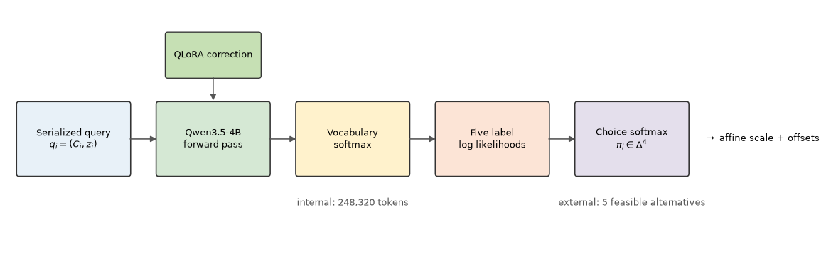
Figure 1. From serialized covariates to a finite-choice probability vector. The vocabulary distribution is internal to the LM; the five-way conditioning and affine map are analyst-imposed.

Adaptation and calibration: features, labels, and losses

This section treats each intervention as an estimator and states its covariates, outcome labels, fitted object, criterion, and sample. The distinction is substantive: ICL consumes labeled observations but fits no persistent parameter; QLoRA estimates millions of network parameters with a vocabulary-level token loss; calibration estimates at most five free numbers from already-produced probabilities.

Labels and the serialized design

Let $J_i\equiv Y_i\in \{1,\dots ,5\}$ denote the displayed position of the candidate with the greatest lifetime playtime and let

$$y_{ij}=1\{J_i=j\}.$$

The complete-suffix estimator uses the canonical strings choice_1 through choice_5. The one-token estimator applies the deterministic verbalizer

$$v(1)=\text{A},v(2)=\text{B},v(3)=\text{C},v(4)=\text{D},v(5)=\text{E}.$$

Thus A means “first displayed candidate,” not a game, brand, or product category. Candidate order is randomized. The 4,000-row estimation pool contains 794, 814, 809, 785, and 798 outcomes at positions one through five. There is no class weighting, oversampling, or label smoothing.

The LM covariate is the literal serialized query $q_i=q(C_i,z_i)$. It contains top non-candidate games and minutes; non-candidate review snippets; ten user-history scalars; and, for each candidate, price, free status, release year, popularity, five history-match measures, title, genres, and tags. Candidate playtime is absent. The single-token specification replaces each canonical position label in the query with its corresponding letter. Appendix B reproduces one complete held-out query and the fitted probability vector from each principal estimator.

The LM is scored at the first admissible answer-token position with no intervening generated tokens. Allowing the model to generate reasoning or other text before the label would define a different classifier whose prediction depends on the generated path.

The frozen and adapted single-token specifications use different fixed instructions. The frozen version describes the model as a “discrete-choice classifier” and appends “Answer with one letter” to each user turn. The adapted version uses the system instruction present during supervised training and does not append that phrase. Demonstrations, verbalizers, and the probability rule are otherwise held fixed in their closest comparison. Consequently, the frozen-to-adapted contrast estimates the joint change in adapter weights and instruction format, not an isolated adapter effect.

In-context conditioning

The five-demonstration specification prepends labeled estimation examples as alternating user and assistant turns. Every demonstration contains the same serialized features and an assistant response $v(J_i)$. The demonstration-selection sample contains the first 256 rows of the randomly permuted estimation split. Within each outcome class, the observation with the shortest serialized query is selected to control context length. This deterministic rule favors observations with relatively sparse histories, and sensitivity to the sample size or demonstration choice is not measured.

Conditional on this rule, ICL estimates no persistent parameter and minimizes no explicit loss:

$$p_{ij}^{\mathrm{ICL}}=p_{{\theta }_0}\{v(j)\mid D,q_i\}.$$

ICL therefore uses five observed outcomes on every prediction, and validation performance determines whether demonstrations are included in the final specification. Demonstrations can communicate the input-output convention even when they do not identify a stable parametric relationship (Min et al. 2022). The reported estimate conditions on this single deterministic demonstration set.

QLoRA estimation

For every adapted attention projection, LoRA replaces a frozen matrix by (Hu et al. 2021)

$$W=W_0+\frac{\alpha }{r}BA,$$

where $A\in {\mathbb{R}}^{r\times d_{\mathrm{in}}}$ and $B\in {\mathbb{R}}^{d_{\mathrm{out}}\times r}$. QLoRA backpropagates through a frozen four-bit base representation while updating only $A$ and $B$ (Dettmers et al. 2023).

Training objective

For row $i$, let $(w_{i1},\dots ,w_{i{T}_i})$ be the tokenized system message, query, and observed assistant completion. Let $R_i$ index unmasked response tokens. Prompt and padding tokens receive the ignore index $-100$. Training minimizes

$${\mathcal{L}}_{\mathrm{SFT}}(A,B)=-\frac{1}{M}\sum _{i\in \mathcal{E}}\sum _{t\in R_i}\log \frac{\exp z_{it,w_{it}}(A,B)}{{\sum }_{u\in \mathcal{V}}\exp z_{it,u}(A,B)},M=\sum _{i\in \mathcal{E}}|R_i|,$$

where $\mathcal{V}$ is Qwen’s entire vocabulary and $\mathcal{E}$ is the 4,000-row estimation pool. An untruncated completion contains three supervised tokens: the outcome letter, Qwen’s end-of-turn marker, and a newline. The same token weight is assigned to all three.

A five-class choice loss would instead use only the outcome-letter position $t_i^{\ast }$ and normalize over the five verbalizers,

$${\mathcal{L}}_5(A,B)=-\frac{1}{|\mathcal{E}|}\sum _{i\in \mathcal{E}}\log \frac{\exp z_{i{t}_i^{\ast },v(J_i)}(A,B)}{{\sum }_{j=1}^5\exp z_{i{t}_i^{\ast },v(j)}(A,B)}.$$

These objectives are not equivalent. At the label position, the vocabulary loss equals the five-class loss plus the log ratio of the full-vocabulary partition function to the five-verbalizer partition function. It also adds two constant-target termination terms. The training loss of 0.5057 therefore cannot be compared with $\log 5$, the validation choice NLL, or the evaluation choice NLL. The termination tokens may become easy quickly, so their share of token count does not measure their share of useful gradient information. A direct restricted-label loss is an important alternative estimator.

Training truncation error

Right truncation at 1,536 tokens removes the response from 22 of 4,000 estimation sequences. The implementation incorrectly places loss on the last available prompt token for these rows rather than on the outcome label. Training ends after 1,600 example presentations, or 0.40 nominal epoch, and minibatch identifiers were not recorded, so the realized optimizer exposure of the 22 affected rows is unknown.

Parameterization and numerical optimization

Component	Specification	Consequence
Frozen training base	NF4, double quantization, BF16 arithmetic	Base weights receive no gradient
Adapter locations	Query, key, value, and output attention projections	Attention only; no MLP projection is adapted
Rank and scale	$r=16$, $\alpha =32$	Training-time multiplier $\alpha /r=2$
Trainable size	3,145,728 of 4.209 billion parameters	0.0747% of model parameters
Regularization	LoRA dropout 0.05; no adapter bias; no weight decay	Stochastic adapter path, zero-initialized through $B$
Optimizer	Paged eight-bit AdamW, learning rate $2\times 10^{-4}$	${\beta }_1=0.9$, ${\beta }_2=0.999$, $ϵ=10^{-8}$, gradient norm at most one
Batching	Effective batch size 8	200 steps equal 1,600 row presentations
Schedule	3% warmup, cosine, seed 42	Adaptive segments ending at 25, 100, and 200 updates

The rank, target projections, and number of updates define the estimator’s capacity. Optimizer precision, clipping, and checkpointing make estimation feasible on a 12 GB GPU. Estimation consists of segments ending at 25, 100, and 200 updates, with continuation determined by validation accuracy. Each segment restarts the cosine schedule, so the learning rate approaches zero at updates 25 and 100 and then rises at the start of the next segment. The resulting learning-rate path differs from a single 200-update cosine decay.

Validation-selected inference setting

At local inference the adapter is applied to a Q4_K_M base rather than the NF4 representation used during training, and it is multiplied by a separate scale $\gamma$,

$$Wh=W_{0}h+\gamma \frac{\alpha }{r}BAh.$$

The checkpoint, $\gamma$, and inclusion of demonstrations are selected sequentially by hard-choice accuracy on the 200-observation validation subsample. The search is non-Cartesian: checkpoint and scale are chosen before demonstrations are added, and the 200-update checkpoint is evaluated only after those earlier choices. Table 3 gives the candidate values and selected specification; Appendix C reports the corresponding validation accuracies.

Table 3. Sequential adapter-model selection on 200 validation observations

Selection dimension	Candidate values	Selected value
Initial checkpoint	25 or 100 updates	100 updates
Adapter scale at 100 updates	$0.5,1,1.25,1.5,2$	$\gamma =1.25$
Demonstrations at 100 updates and $\gamma =1.25$	zero or five	five
Final checkpoint with five demonstrations and $\gamma =1.25$	100 or 200 updates	200 updates

For a proportion near one-half, the binomial standard error at $N=200$ is about 0.035. The selected settings are therefore noisy estimates of nearby alternatives. The search is sequential rather than Cartesian, has no multiplicity correction, and reuses the same 200 observations within the 1,000-row calibration sample. These features create validation-selection optimism.

The distinction between $\gamma$ and calibration temperature is important. $\gamma =1.25$ amplifies the estimated neural update before the network produces logits; $T$ rescales log probabilities after the network has produced a five-vector. They need not have the same empirical effect.

Economic interpretation of the low-rank restriction

Write the task-specific index as

$$V_{ij}^{\ast }=V_{ij}^0+G_{ij},$$

where $V_{ij}^0$ is the frozen LM index and $G_{ij}$ is the correction required for this outcome. Pretraining may already represent semantic similarity, genre, popularity, and history-candidate match; adaptation changes how those represented signals map into the revealed-use label. A useful low-dimensional hypothesis is

$$G_{ij}\approx \sum _{\ell =1}^R{s}_{\ell }(C_i,z_i,j){\lambda }_{\ell }.$$

Possible directions include affinity with high-playtime history, multiplayer fit, novelty, and generic popularity. These names are economic interpretations, not identified adapter factors, and the interpretive dimension $R$ need not equal the matrix rank $r$.

A local expansion gives

$$V_{ij}({\theta }_0+\Delta \theta )\approx V_{ij}({\theta }_0)+g_{ij}^{\top }\mathrm{vec}(\Delta \theta ).$$

Because $\Delta \theta$ is restricted to low-rank changes in selected matrices, the allowable index correction lies in a restricted tangent family. That is the useful analogy to low-dimensional mixed-logit heterogeneity. It is not an equivalence: QLoRA estimates no distribution $F({\beta }_i)$, its heterogeneity is deterministic conditional on the query, and rank 16 in neural weight space does not imply a rank-16 user-item utility matrix.

Frozen likelihood renormalization and calibration

Calibration is fitted separately for each raw LM probability source. Let $p_i=(p_{i1},\dots ,p_{i5})$ denote the source vector and define

$${\check{p}}_{ij}=\frac{\max \{p_{ij},10^{-12}\}}{{\sum }_{k=1}^5\max \{p_{ik},10^{-12}\}},x_{ij}=\log {\check{p}}_{ij}.$$

The only calibrator covariates are the five logged source probabilities $x_i$. No Steam field, text embedding, user identity, or candidate identity enters. The target is the same $y_{ij}$, and the common criterion is multiclass negative log likelihood,

$${\mathcal{L}}_{\mathrm{NLL}}(\eta ;\mathcal{I})=-\frac{1}{|\mathcal{I}|}\sum _{i\in \mathcal{I}}\sum _{j=1}^5{y}_{ij}\log q_{ij}(\eta ).$$

Five stratified folds split the 1,000 validation observations, with shuffling and seed 42. Parameters are fitted on 800 rows and scored on the other 200; the concatenated holdouts provide out-of-fold selection metrics for the calibrator. The upstream adapter specification has already been selected using 200 observations from this same validation sample, so these are not end-to-end out-of-sample metrics. The selected calibration family is then refitted on all 1,000 validation rows and applied once to test.

The four candidate maps are:

1. Direct: $q_{ij}={\check{p}}_{ij}$; no fitted parameter.
2. Temperature: $q_{ij}={\mathrm{softmax}}_j(x_{ij}/T)$ with $T=\exp (\tau )>0$, estimated by minimizing NLL. Because division by a common positive number preserves ordering, temperature alone cannot change accuracy. The selected adapted source gives full-validation $T=0.8589$.
3. Marginal prior shift: $q_{ij}={\mathrm{softmax}}_j(x_{ij}+\lambda d_j)$, where $d_j=\log {\bar{y}}_j-\log {\bar{p}}_j$. Both moments and $\lambda \in \{0,0.025,\dots ,2\}$ are recomputed inside every training fold. Unlike the other fitted calibration families, this exploratory comparator selects $\lambda$ by training-fold accuracy. The full-validation values are $\lambda =1.15$ and $d=(0.406,-0.026,-0.122,-0.170,0.011)$.
4. Affine:

$$q_{ij}^{\mathrm{affine}}={\mathrm{softmax}}_j\left(\frac{x_{ij}}{\exp (\tau )}+b_j\right),\sum _{j=1}^5{b}_j=0.$$

Affine calibration is a conditional logit with one alternative-varying regressor $x_{ij}$, a common slope $1/T$, and four identified alternative-specific constants. Its criterion is

$${\mathcal{Q}}_{\mathrm{affine}}={\mathcal{L}}_{\mathrm{NLL}}+10^{-3}\sum _{j=1}^5{b}_j^2;$$

the common slope is unpenalized. For the selected adapted source, the full-validation fit is $T=0.7772$ and

$$b=(0.541,-0.063,-0.204,-0.251,-0.023).$$

Because displayed positions are randomized, these offsets are not product constants or tastes. They measure systematic distortion associated with letter and display position. The positive first-position adjustment and broadly decreasing offsets through position four are consistent with prompt or verbalizer position bias, a known issue in few-shot classification (Zhao et al. 2021). Deterministic tie-breaking could also favor position one, but only one observation in the entire validation split has a tied maximum, so it cannot mechanically account for an offset affecting the full sample. The partial recovery at position five cautions against a literal linear primacy story.

The estimate $T<1$ sharpens rather than flattens probabilities, implying that the raw adapted model is underconfident on validation. Calibration improves predictive probabilities (Guo et al. 2017); it does not recover preference coefficients. Appendix C gives optimizer initialization, parameter encoding, and deterministic tie rules for the calibration computations.

Exploratory activation steering

Activation steering tests whether a single supervised displacement of the model’s hidden state can change candidate rankings without updating network weights. This restriction is substantially narrower than QLoRA because the same direction is applied to every query, candidate, and token position. It changes confidence slightly but does not materially improve validation classification, so no steering specification is calibrated or evaluated on test. Appendix A defines the features, labels, auxiliary probe, contrast direction, and scale comparison.

Evaluation

Accuracy is the principal hard-classification statistic because it is the only performance object shared by the local probability estimators and the external hard-label classifiers. The empirical position-frequency baseline is 0.205, close to but not exactly the theoretical 0.200 chance rate. Macro F1 prevents a favorable aggregate score from hiding a failed displayed position.

For systems that return a probability vector, average negative log likelihood is the primary probability criterion,

$$\mathrm{NLL}=-\frac{1}{N}\sum _{i=1}^N\log {\hat{\pi }}_{i{Y}_i}.$$

It is a strictly proper score and directly punishes assigning little mass to the realized alternative. The multiclass Brier score is the mean squared distance from the one-hot outcome and is less tail-sensitive. One-versus-rest macro AUC measures ranking separately for each displayed position and does not evaluate calibration.

Model and adapter settings use validation outcomes, and calibration families use five-fold out-of-fold predictions from the same validation sample before a full-validation refit. Marginal 95% Wilson intervals accompany accuracy points in the figure. Differences use 100,000 paired nonparametric bootstrap resamples of the 1,000 test observations; because each row belongs to a distinct user, this also resamples users. Exact two-sided McNemar tests use the two discordant cell counts.

Results

Comparative predictive performance

Table 4 evaluates the simple rules, classical probability estimators, and local LM specifications on the same 1,000 observations. Symmetric conditional logit is the primary benchmark because candidate position is randomized and its common coefficients respect alternative exchangeability. It reaches 0.461 accuracy and has the best NLL, Brier score, and AUC in the table. The calibrated Qwen specification has the highest hard-accuracy point estimate, 0.480, but its NLL is 0.010 higher.

Table 4. Test performance on 1,000 common observations

Estimator	Accuracy	Macro F1	NLL	Brier	Macro AUC
Position-frequency prior	0.205	0.068	1.609	0.800	0.500
Most-popular candidate	0.404	0.404	–	–	–
Identity-based low-rank logit, rank 2	0.287	0.286	2.942	0.965	0.539
Pooled position classifier, 1,180 fitted numbers	0.416	0.417	1.450	0.720	0.727
Symmetric conditional logit, 45 attributes	0.461	0.461	1.335	0.671	0.754
Frozen Qwen, complete-suffix likelihood	0.286	0.282	1.839	0.878	0.601
Frozen Qwen, five-shot one-token likelihood	0.286	0.273	1.830	0.884	0.615
Frozen Qwen, five-shot plus affine calibration	0.308	0.308	1.557	0.778	0.619
Adapted Qwen, training-format instruction and five-shot, uncalibrated	0.462	0.460	1.381	0.689	0.751
Adapted Qwen plus affine calibration	0.480	0.480	1.345	0.673	0.751

The popularity rule is included only as a hard decision rule; because it estimates no probability model, proper scores are omitted. The two frozen rows differ in both label representation and demonstrations, so their equal accuracy does not identify an ICL effect.

The closest frozen-to-adapted comparison holds the one-token verbalizers and five demonstrations fixed but jointly changes chat formatting and adapter weights, as detailed in the methods. Accuracy rises from 0.286 to 0.462 across that joint change. The 17.6-point contrast therefore measures the adapted specification as a whole rather than the adapter’s isolated contribution. Independently fitted affine models move the corresponding final figures from 0.308 to 0.480.

The identity factor model performs poorly in this sparse design. There are only 1.34 estimation observations per represented user, and 263 test users are absent from estimation. Its rank-two factors therefore have little repeated-choice information from which to learn, while the most-frequent-user substitution supplies no individualized information for absent users. This result characterizes the present data regime rather than matrix-completion choice models generally.

Paired comparisons

Table 5 compares calibrated Qwen with three references. Its 6.4-point advantage over the pooled position classifier remains positive under paired resampling. The primary conditional-logit comparison is much closer: the point difference is 1.9 points, its interval includes zero, and the exact discordance test does not reject equality.

Table 5. Paired test comparisons for selected Qwen

Reference	Reference accuracy	Qwen minus reference	Paired bootstrap 95% interval	Qwen only correct	Reference only correct	Exact McNemar $p$
Most-popular candidate	0.404	0.076	$[0.044,0.108]$	177	101	$6.0\times 10^{-6}$
Pooled position classifier	0.416	0.064	$[0.033,0.095]$	159	95	$7.1\times 10^{-5}$
Symmetric conditional logit	0.461	0.019	$[-0.007,0.045]$	100	81	0.181

For the main conditional-logit comparison, Qwen NLL minus conditional-logit NLL is 0.010, with paired bootstrap interval $[-0.017,0.037]$. Thus neither the accuracy evidence nor the proper-score evidence establishes dominance. The 181 rows on which exactly one of these two systems is correct are nevertheless informative: the systems are not duplicates, and a validation-designed ensemble is a natural next experiment.

External hard-label classifiers

The three API configurations cover the same 1,000 test observations. They use the same serialized information and target positions, but only generated labels are available. GPT-5.3 Codex Spark uses xhigh reasoning with zero or one demonstration; GPT-5.5 uses medium reasoning with five. Neither receives task-specific parameter updates.

Table 6. Hard-label classification on the common test sample

Prediction system	Task-specific parameter fitting	Demonstrations	Accuracy	Macro F1	Parseable output
Selected local Qwen3.5-4B	3.15-million-parameter QLoRA adapter plus five-parameter affine map	5	0.480	0.480	1.000
Symmetric conditional logit	45-coefficient penalized likelihood	0	0.461	0.461	1.000
Pooled position classifier	1,180 fitted numbers	0	0.416	0.417	1.000
GPT-5.5, medium reasoning	None	5	0.387	0.388	1.000
GPT-5.3 Codex Spark, xhigh	None	0	0.272	0.272	0.996
GPT-5.3 Codex Spark, xhigh	None	1	0.260	0.260	0.992

Malformed or missing API labels count as incorrect: four Spark zero-demonstration rows and eight one-demonstration rows are invalid. Five-demonstration GPT-5.5 is 7.4 points below conditional logit and 9.3 points below adapted Qwen. The comparison is asymmetric in task information: Qwen receives 1,600 optimizer presentations drawn from 4,000 labeled rows, whereas GPT-5.5 receives five labels in context. These figures compare complete task-specific procedures, not general model capability. The 1.2-point Spark difference also changes the context and one demonstration and is too small to support a general conclusion about ICL.

Figure 2 collects the principal local specifications, the classical benchmarks, and the three full-sample API configurations. Every point has the same denominator and observation identifiers.

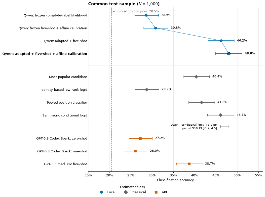
Figure 2. Hard-choice accuracy on the same 1,000 test observations. The adapted Qwen labels denote the joint QLoRA, instruction-format, and demonstration specification. Bars are marginal 95% Wilson intervals. The bracket emphasizes the paired Qwen versus conditional-logit comparison; its interval is for the paired difference, not the marginal bars. Invalid API outputs count as incorrect.

User overlap

Table 7 stratifies the same test sample by whether the user’s identifier appears in the 4,000-observation estimation sample. Every estimator except the identity-factor model continues to use observed attributes or the serialized history for users not represented in estimation.

Table 7. Accuracy by user overlap with the 4,000-observation estimation sample

Test group	$N$	Popularity	Identity low-rank	Pooled classifier	Conditional logit	Selected Qwen
User represented	737	0.406	0.290	0.408	0.459	0.463
User absent	263	0.399	0.285	0.437	0.468	0.529

The Qwen-minus-conditional-logit difference is 6.1 points among users absent from the 4,000-observation estimation sample and 0.4 points among represented users. User identifiers never enter Qwen, so direct identifier memorization cannot generate this pattern. The comparison remains descriptive: the groups differ compositionally, every row contains a non-candidate history, and no subgroup-specific specification was selected.

What calibration changes

Affine calibration is selected because it has the best calibrator-only out-of-fold validation accuracy, NLL, and Brier score. Prior shift classifies one additional test row, but calibration-family selection is based on validation data. Affine calibration also has the lower test NLL.

Table 8. Adapted-model calibration

Transformation	Calibrator-only OOF accuracy	Calibrator-only OOF NLL	Test accuracy	Test NLL	Test Brier
Direct	0.445	1.388	0.462	1.381	0.689
Temperature	0.445	1.388	0.462	1.378	0.685
Prior shift	0.444	1.370	0.481	1.356	0.679
Affine	0.451	1.361	0.480	1.345	0.673

Figure 3 compares top-choice confidence with realized top-choice accuracy in five equal-count test bins. This diagnostic is descriptive because the same test outcomes define the displayed reliability points; calibration parameters themselves were estimated only on validation. Affine calibration lowers this top-choice expected calibration error from 0.063 to 0.037.

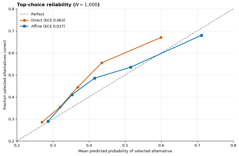
Figure 3. Top-choice reliability before and after affine calibration. Each point contains 200 test observations; the diagonal is perfect calibration. ECE is the equal-count-bin weighted absolute confidence gap.

Quantization robustness

The deployment specification uses Q4_K_M base weights. A fixed BF16 evaluation applies the same 200-update adapter, scale 1.25, demonstrations, grammar, test identifiers, and Q4-estimated affine calibration. No component is retuned under BF16.

Table 9. Q4_K_M and BF16 inference parity

Base and probability map	Accuracy	Macro F1	NLL	Brier	Macro AUC
Q4_K_M, raw	0.462	0.460	1.381	0.689	0.751
BF16, raw	0.462	0.462	1.370	0.683	0.753
Q4_K_M, validation-fitted affine	0.480	0.480	1.345	0.673	0.751
BF16, same fixed Q4 affine map	0.477	0.477	1.345	0.671	0.753

Aggregate performance is stable, but the two numerical representations are not rowwise identical. Raw argmax agreement is 0.908 and affine argmax agreement is 0.910. Mean absolute probability difference is 0.0195, mean rowwise total-variation distance is 0.0487, and gold-probability correlation is 0.984. Raw Q4-minus-BF16 accuracy is exactly zero with paired interval $[-0.014,0.014]$; under the fixed affine map it is 0.003 with interval $[-0.011,0.017]$. The result supports Q4 deployment at the aggregate level while warning against treating quantization as bitwise or observation-level invariance.

Computational requirements

All local LM results use an NVIDIA RTX 5070 with 12 GB of memory. The Q4_K_M base is 3.01 GB and the selected adapter is 6.29 MB; the BF16 base is approximately 8.4 GB. Table 10 reports fitting, model-selection, and scoring time separately.

Table 10. Recorded compute

Operation	Sample or passes	Recorded time	Qualification
Conditional-logit ridge grid	6 fits on 4,000 rows	0.42 s CPU cumulative	Selected fit itself takes 0.07 s
Identity low-rank rank/penalty grid	16 fits on 4,000 rows	88.6 s CPU cumulative	Selected fit itself takes 3.80 s
Pooled-classifier fit	4,000 rows	7.93 s CPU	235 standardized covariates and five logits
QLoRA updates 101–200	100 updates	624.5 s GPU	Total adapter-training time is unavailable
Adapter-model selection	9 evaluation passes of 200 rows	about 781 s GPU	Sequential validation search
Frozen complete-suffix test scoring	1,000 rows	218.1 s GPU	4.59 rows/s; common-prefix branching
Selected Q4 validation scoring	1,000 rows	447.9 s GPU	Five demonstrations
Selected Q4 test scoring	1,000 rows	450.8 s GPU	2.22 rows/s
Fixed BF16 test scoring	1,000 rows	384.6 s GPU	No component retuned

The median selected-model prompt has 5,616 tokens, and llama.cpp reuses a median 4,639 cached prompt tokens from the fixed demonstrations. At the observed Q4 rate, one million similarly sized choice occasions would require roughly 125 serial GPU-hours before engineering for parallel devices or batching. The local method is feasible, not free. Conditional logit is the obvious operational default when its hand-built feature map is adequate; the local LM buys a text-native representation at several orders of magnitude more computation.

Interpretation

The results support four conclusions.

First, symmetry matters more than model branding. The pooled position classifier wastes parameters by learning five versions of relationships that should be exchangeable. The 45-coefficient conditional logit improves its accuracy by 4.5 points and NLL by 0.115. It essentially matches the uncalibrated adapted Qwen specification and slightly outperforms the final LM on every reported probability score. For an analyst who already has the 45 candidate attributes, conditional logit is the best default here.

Second, pretrained representation is not outcome alignment. Frozen Qwen is weak despite seeing titles, tags, histories, and reviews. The jointly adapted specification, which introduces outcome-supervised low-rank weights together with the training-format instruction, is much more accurate. This pattern is consistent with a restricted correction $G_{ij}$ to represented signals, but the formatting difference prevents attribution of the full 17.6-point contrast to adapter weights alone. The fitted correction also does not reveal whether the predictive signal is “taste,” popularity, genre duration, or another regularity.

Third, calibration is a small econometric model, not cosmetic post-processing. The affine layer estimates a common log-probability slope and position constants. It adds 1.8 accuracy points, materially improves reliability, and exposes a large first-position measurement offset. Those gains should be attributed to validation labels and five fitted calibration degrees of freedom, not to the base LM.

Fourth, the LM and conditional logit are complements before they are rivals. Qwen is uniquely correct on 100 rows and conditional logit on 81. A combined model could use the conditional index, LM index, or both as alternative-varying regressors and estimate their weights on validation data. That design would test whether text contributes beyond the structured attribute benchmark while explicitly accounting for their different information sets.

The external comparisons reinforce the importance of task information. A general-purpose model with five demonstrations is not matched on training exposure to a local model receiving 1,600 presentations from a 4,000-row labeled pool. Its lower accuracy is consistent with a benefit from persistent task estimation; it does not rank general intelligence. Similarly, the popularity baseline shows that a nontrivial share of the task is generic item comparison. Separating popularity, semantic match, and individualization requires item-held-out evaluation and targeted feature ablations.

An operational decision rule follows. Use conditional logit when the alternative attributes are available and probability quality, speed, or interpretability matter. Add a local adapter when important information is genuinely textual, the same narrow outcome recurs often enough to amortize training, and a held-out gain persists relative to a symmetric benchmark. Use calibration whenever probabilities rather than only rankings matter. Do not use this fitted index for price elasticities, welfare, assortment counterfactuals, or policy simulation without a separate behavioral and identification argument.

Limitations

The first limitation is the estimand. Highest lifetime playtime among five already-owned games is a revealed-use ranking, not a purchase at a known menu. It combines preference, exposure, ownership duration, and genre-specific time intensity.

Second, the alternatives are analyst-sampled from a 500-game catalog. Probabilities are conditional on that sampled set and cannot be aggregated into market shares without modeling the sampling and availability process. Catalog rank and popularity are computed from the first 30,000 source user records before splitting, so the experiment is transductive with respect to those product-level fields.

Third, the study is retrospective and not preregistered. Computational caps were chosen during development, and preliminary tuning, including selection of the API configurations, inspected smaller test-split subsets. The reported intervals are therefore descriptive for this realized 1,000-observation analysis. They omit uncertainty from adapter training, demonstration choice, validation search, calibration estimation, instruction design, quantization, and base-model pretraining.

Fourth, demonstration selection and adapter estimation are measured only once. Demonstrations are selected deterministically by minimum serialized length within the 256-observation selection sample. There is no random-demonstration distribution, item-held-out evaluation, independent adapter seed, or repeated fit.

Fifth, standard SFT does not optimize the reported five-way likelihood. Two of three intended response tokens are chat termination material, and 22 right-truncated estimation rows lose the label entirely. The adaptive training schedule covers only 1,600 example presentations and restarts its cosine schedule twice. Convergence to either the vocabulary objective or the ideal five-class objective is not assessed.

Sixth, complete prediction systems receive different representations. Conditional logit receives 45 engineered candidate attributes; Qwen receives a textual serialization containing some of those values plus titles, tags, and reviews. Qwen also uses five labels in context and 1,600 stochastic example presentations, whereas the classical estimators use all 4,000 labels directly. The comparison does not isolate functional form, text, or effective sample size. Moreover, the closest frozen and adapted LM specifications use different chat instructions, so their accuracy difference does not isolate QLoRA.

Seventh, user overlap is not randomly assigned. The stronger point accuracy among users absent from the 4,000-observation estimation sample may reflect composition and does not establish cold-start superiority. The identity-based low-rank result is especially sensitive to sparse observations per user and its ad hoc absent-user substitution.

Eighth, the study covers one dataset, one four-billion-parameter architecture, one adapter parameterization, one Q4 format, and one GPU. The BF16 comparison supports aggregate quantization robustness for this specification, not a general invariance claim. The three API configurations are not an exhaustive comparison of external models.

Finally, finite-set normalization creates coherent predictive probabilities but not a structural random-utility model. The LM index can depend on the entire prompt, displayed order, and arbitrary verbalizers; it need not satisfy regularity or stable substitution restrictions. Endogenous price, exposure, and assortment remain endogenous after passing through a neural network. Instruments, experimental variation, supply-side structure, or explicit assignment assumptions are still required for causal demand analysis.

Conclusion

A quantized four-billion-parameter LM can be converted into a finite-choice probability estimator by scoring admissible labels and conditioning on the displayed set. Frozen likelihoods are not competitive in this application. A jointly adapted specification combining a 3.15-million-parameter QLoRA adapter, the training-format instruction, and five demonstrations supplies the large improvement. The separate test-sample contribution of demonstrations and instruction wording is not identified. A five-parameter affine layer adds 1.8 accuracy points and improves probability alignment.

The resulting 0.480 test accuracy is higher than the popularity rule, the pooled position classifier, conditional logit, and the three full-sample API configurations. Symmetric conditional logit already reaches 0.461 and has slightly better NLL, Brier score, and AUC. The 1.9-point paired accuracy difference is not statistically distinguishable from zero under test-sample resampling. The local model is therefore competitive with a strong conventional estimator, not shown to dominate it.

For empirical economists, the useful object is a nonlinear systematic-index engine whose label use and loss function can be stated explicitly. Frozen scoring exposes the pretrained index; ICL conditions it on labeled vignettes; QLoRA estimates a restricted domain correction; affine calibration estimates a familiar scale and alternative-specific constants. Neural low rank is a regularizer in parameter space, not identified low-dimensional taste heterogeneity. The method is promising for recurring text-rich prediction problems when evaluated against an exchangeable choice model and interpreted as prediction rather than structural demand.

Appendix A: Activation-steering diagnostic

Activation steering (Turner et al. 2024) is evaluated as a weight-preserving alternative to parameter adaptation. An auxiliary probe selects a transformer block. The probe uses 1,000 observations from each of the permuted estimation and validation splits; its features are the standardized final-query hidden state ${\tilde{h}}_{i\ell }$ of the frozen model, and its labels are the same five position outcomes $y_{ij}$. At candidate block $\ell$, penalized multinomial logistic regression estimates intercepts and class coefficients by minimizing

$${\mathcal{Q}}_{\mathrm{probe}}(a,\beta ;\ell ,C)=-\frac{1}{1000}\sum _{i=1}^{1000}\sum _{j=1}^5{y}_{ij}\log {\rho }_{ij}(a,\beta ;\ell )+\frac{1}{2C(1000)}\sum _{j=1}^5\Vert {\beta }_j{\Vert }_2^2,$$

where

$${\rho }_{ij}(a,\beta ;\ell )={\mathrm{softmax}}_j\left(a_j+{\tilde{h}}_{i\ell }^{\top }{\beta }_j\right).$$

Intercepts are unpenalized. Blocks 24, 28, and 31 sample three depths in the upper quarter of the 32-block network; no exhaustive layer search is performed. Values $C\in \{0.01,0.1,1,10\}$ are compared by accuracy on 1,000 validation rows after fitting on 1,000 estimation rows. Block 24 with $C=0.01$ reaches 0.267, versus maxima 0.237 and 0.240 at blocks 28 and 31. The probe is used only for layer selection.

The direction uses a separate supervised contrast. Let ${\bar{h}}_{i\ell }(j)$ be the layer-$\ell$ hidden state averaged over the complete response-suffix tokens after presenting query $q_i$ and candidate response choice_j. Define the cyclic counterlabel $c(j)=j+1$ for $j<5$ and $c(5)=1$. On the 1,000-observation estimation sample,

$$r_{\ell }=\frac{1}{1000}\sum _{i=1}^{1000}\left\{{\bar{h}}_{i\ell }(J_i)-{\bar{h}}_{i\ell }[c(J_i)]\right\},v_{\ell }=\frac{r_{\ell }}{\Vert r_{\ell }{\Vert }_2}.$$

The feature is therefore the frozen hidden state induced by the serialized covariates; $J_i$ supplies the positive suffix and the cyclic label supplies the negative suffix. No classifier or differentiable loss fits $v_{\ell }$: it is a difference of sample means followed by normalization. The source is frozen Q4 Qwen with maximum sequence length 6,144. The same intervention is added at every token position in block 24,

$$h_{i,24,t}^{\prime }=h_{i,24,t}+\gamma v_{24}.$$

Scales are compared on the 200-observation validation subsample used for adapter-model selection. Because steering does not materially improve classification, it is not evaluated on the test sample.

Steering scale $\gamma$	Accuracy	Macro F1	NLL	Macro AUC
0	0.320	0.301	1.937	0.572
-2	0.325	0.305	1.889	0.569
-4	0.325	0.305	1.853	0.567
-8	0.320	0.293	1.812	0.566

The direction changes confidence but not classification materially and degrades AUC monotonically. A single alternative-agnostic vector applied to every token is too restrictive to supply the candidate-specific correction learned by QLoRA.

Appendix B: Illustrative serialized observation

The following query is one held-out observation after deterministic replacement of choice_1 through choice_5 by A through E. Line wrapping is the only change from the model input. Its observation identifier is 12678.

SYSTEM: You are a discrete choice model. Given structured covariates and
candidate alternatives, predict the observed chosen alternative. Respond
with exactly one label from: A, B, C, D, E.
 
USER: Predict which held-out Steam game this user played the most.
The observed user history below excludes all candidate games and candidate reviews.
Return exactly one label from: A, B, C, D, E.
 
Top played non-candidate games as [game, lifetime playtime minutes; ...]:
[Warframe, 8559; Terraria, 5410; Euro Truck Simulator 2, 2674;
 Don't Starve Together, 492; PAYDAY 2, 186; Counter-Strike: Source, 149;
 Fractured Space, 104;
 Red Orchestra 2: Heroes of Stalingrad with Rising Storm, 48]
 
Non-candidate reviews as [game, recommended flag, review text; ...]:
[none]
 
Tabular features:
- user: user_items_count=51, user_played_games=28, history_played_games=8,
  history_total_playtime=17622, history_mean_playtime=2202.75,
  history_median_playtime=339, history_max_playtime=8559,
  history_review_count=0, history_recommend_share=0,
  history_mean_review_length=0
- A: price=0, is_free=1, release_year=2017, popularity_count=13970,
  popularity_rank=4, history_term_minute_score=7.34,
  history_term_count_score=57, history_term_overlap=13,
  history_developer_match_count=0, history_publisher_match_count=0
- B: price=0.99, is_free=0, release_year=2013, popularity_count=3430,
  popularity_rank=66, history_term_minute_score=7.17,
  history_term_count_score=55, history_term_overlap=11,
  history_developer_match_count=0, history_publisher_match_count=0
- C: price=0, is_free=1, release_year=2011, popularity_count=4863,
  popularity_rank=39, history_term_minute_score=6.2,
  history_term_count_score=49, history_term_overlap=11,
  history_developer_match_count=0, history_publisher_match_count=0
- D: price=19.99, is_free=0, release_year=2015, popularity_count=6368,
  popularity_rank=18, history_term_minute_score=4.53,
  history_term_count_score=37, history_term_overlap=9,
  history_developer_match_count=0, history_publisher_match_count=0
- E: price=39.99, is_free=0, release_year=2015, popularity_count=4949,
  popularity_rank=37, history_term_minute_score=6.83,
  history_term_count_score=53, history_term_overlap=12,
  history_developer_match_count=0, history_publisher_match_count=0
 
Candidate games:
- A: Unturned | genres: Action, Adventure, Casual, Free to Play |
  tags: Free to Play, Survival, Zombies, Multiplayer, Open World, Adventure |
  price: 0 | release year: 2017
- B: ORION: Prelude | genres: Action, Adventure, Indie, RPG |
  tags: Dinosaurs, Action, FPS, Multiplayer, Online Co-Op, Co-op |
  price: 0.99 | release year: 2013
- C: No More Room in Hell | genres: Action, Free to Play, Indie |
  tags: Free to Play, Zombies, Multiplayer, Survival, Horror, Co-op |
  price: 0 | release year: 2011
- D: Rocket League® | genres: Action, Indie, Racing, Sports |
  tags: Multiplayer, Racing, Soccer, Sports, Competitive, Team-Based |
  price: 19.99 | release year: 2015
- E: Grand Theft Auto V | genres: Action, Adventure |
  tags: Open World, Action, Multiplayer, First-Person, Third Person, Crime |
  price: 39.99 | release year: 2015
 
Answer with only the label.

The observed outcome is E. The fitted choice probabilities for this held-out query are:

Estimator	$p(A)$	$p(B)$	$p(C)$	$p(D)$	$p(E)$	Prediction
Frozen full-label scoring	0.536	0.019	0.412	0.020	0.013	A
Frozen single-token scoring, five demonstrations	0.371	0.135	0.291	0.134	0.070	A
Adapted Qwen, uncalibrated	0.041	0.046	0.049	0.201	0.662	E
Adapted Qwen plus affine calibration	0.039	0.024	0.023	0.134	0.780	E
Conditional logit	0.206	0.098	0.044	0.204	0.448	E

Appendix C: Reproducibility protocol

The public discrete-choice-finetune repository contains the article source, locked software environment, data-construction and estimation code, processed-data metadata, row-level predictions, and result tables. The folded cells below connect the empirical definitions to executable implementations. Rendering from the deposited results requires no model or external request; reconstructing model outputs requires the raw Steam files, model weights, and GPU resources described in the repository README.

The model and software identities are:

Component	Version or identifier	Reproducibility record
Adapter-training base	Qwen/Qwen3.5-4B, Hugging Face snapshot 851bf6e806efd8d0a36b00ddf55e13ccb7b8cd0a	PyTorch 2.9.1+cu128; Transformers 5.6.0.dev0; PEFT 0.18.1; bitsandbytes 0.48.2
Local inference base	Qwen3.5-4B Q4_K_M GGUF	SHA-256 13c16f426047e2de38cd075bdade4a7bcbc8c774384876f677740cda65f8a983
Selected adapter	200-update F16 LoRA GGUF	SHA-256 eebd309aad26c9f305e28a0324588c6948d6e7e60206152c2b7e2a286e37b82c
Local inference runtime	llama.cpp version 1458, commit 720d7fa4097f76e5d0eade5a92c1df87c1faf9d9	GNU 13.3.0 Linux x86-64 build
External-model interface	OpenAI Codex CLI 0.145.0, ephemeral read-only structured-output execution	Model identifiers gpt-5.3-codex-spark and gpt-5.5; provider snapshots were not exposed by the interface
Article environment	Python 3.12.11; NumPy 2.4.4; pandas 2.3.3; scikit-learn 1.8.0; Quarto 1.5.57	Locked by uv.lock

The deterministic demonstration and external-call settings are:

Estimator	Demonstration observation identifiers and outcomes	Selection sample	Additional setting
Local single-token and adapted Qwen	9944 (A), 2952 (B), 14726 (C), 12676 (D), 14087 (E)	First 256 rows of the permuted estimation split; shortest within class	Five demonstrations
GPT-5.3 Codex Spark	None	–	Zero demonstrations; xhigh; batch size 20
GPT-5.3 Codex Spark	6728 (choice_1)	First 1,000 rows of the permuted estimation split; first class-balanced match	One demonstration; xhigh; batch size 20
GPT-5.5	6728, 13617, 6964, 2927, 4388 (choice_1–choice_5)	First 1,000 rows of the permuted estimation split; first class-balanced matches	Five demonstrations; medium; batch size 5

The three complete API evaluations were finalized on July 26, 2026. Each batch was submitted through codex exec with a JSON schema restricting outputs to an array of observation identifiers and choice_1–choice_5 labels. The fixed instruction identified the task as discrete-choice evaluation, prohibited tools and file or web access, required one prediction for every held-out identifier, and required schema-conforming JSON. Temperature and top-$p$ controls were not exposed by this interface. The deposited API table contains observation identifiers, gold labels, parsed predictions, validity indicators, and run settings; raw response payloads are not deposited.

The sequential adapter-model search produced the following validation accuracies:

Selection dimension	Fixed components	Candidate accuracies	Selected value
Initial checkpoint	$\gamma =1$, no demonstrations	25 updates: 0.385; 100 updates: 0.440	100 updates
Adapter scale	100 updates, no demonstrations	0.5: 0.395; 1: 0.440; 1.25: 0.470; 1.5: 0.445; 2: 0.420	$\gamma =1.25$
Demonstrations	100 updates, $\gamma =1.25$	zero: 0.470; five: 0.495	five
Final checkpoint	five demonstrations, $\gamma =1.25$	100 updates: 0.495; 200 updates: 0.500	200 updates

For the identity-factor grid, validation ties are resolved by NLL, root-mean-squared probability error, Brier score, macro F1, and macro AUC, in that order; an exact tie then follows ascending rank and penalty. For marginal prior-shift calibration, training-fold accuracy ties are resolved by NLL and then larger $\lambda$. Temperature and affine optimization begin at $T=1$ and zero offsets. The affine implementation uses four unrestricted offset parameters, appends a fifth zero, and centers the five-vector to enforce ${\sum }_j{b}_j=0$.

Data construction and split validation

The data procedure constructs disjoint candidate sets, excludes candidate outcomes from the covariates, applies the within-user randomization with seed 42, and verifies labels against the common choice table.

split	observations	users
train	7845	4078
validation	4078	4078
test	4078	4078

Classical estimation

The classical procedure fits the pooled position classifier, symmetric conditional logit, and identity-based low-rank logit on the 4,000-observation estimation sample. It records feature definitions, validation grids, selected penalties or rank, and row-level validation and test probabilities.

model	accuracy	macro_f1	log_loss
pooled position classifier	0.416	0.417	1.450
symmetric conditional logit	0.461	0.461	1.335
identity-based low-rank logit	0.287	0.286	2.942

Frozen full-label scoring

The scoring procedure branches after the common query, sums the autoregressive log likelihood of every complete response suffix, and applies the five-way choice softmax.

estimator	test_accuracy	test_macro_f1	test_log_loss	test_brier
complete finite-label likelihood	0.286	0.282	1.839	0.878

In-context conditioning

Five short, class-balanced estimation cases are serialized as alternating user and assistant turns. The response grammar permits only the one-token verbalizers A–E; classification uses the returned token probabilities, not the sampled token.

estimator	test_accuracy	test_macro_f1	test_log_loss	test_brier
five-example one-token likelihood	0.286	0.273	1.830	0.884

QLoRA estimation and scoring

The adaptive rank-16 optimization produces checkpoints after 25, 100, and 200 updates. The 200-update adapter is applied at validation-selected scale 1.25 and evaluated with the same five demonstrations and single-token probability rule.

estimator	test_accuracy	test_macro_f1	test_log_loss	test_brier
rank-16 adapter plus five examples	0.462	0.460	1.381	0.689

Probability calibration

No network parameter is updated here. For each estimator, validation probabilities and labels fit temperature, prior-shift, and affine transformations. Five-fold out-of-fold validation metrics select the reported transformation; the selected map is then refitted on all validation observations and applied once to test probabilities.

estimator	test_accuracy	test_macro_f1	test_log_loss	test_brier
rank-16 adapter plus five examples and affine calibration	0.480	0.480	1.345	0.673

Activation-steering diagnostic

The steering procedure estimates a global contrast direction from 1,000 observations in the permuted estimation split at transformer block 24 and applies it at every token position. The 200-observation validation subsample compares scales $-2$, $-4$, and $-8$; the test sample is not scored.

estimator	validation_accuracy	validation_log_loss
unsteered complete finite-label likelihood	0.320	1.937
global layer 24 all-token scale -2	0.325	1.889
global layer 24 all-token scale -4	0.325	1.853
global layer 24 all-token scale -8	0.320	1.812

Numerical verification

The final cell checks the principal numerical claims against the deposited result tables, paired comparisons, quantization summary, and API decision tables. It performs no model fitting or external request.

All numerical consistency checks passed.

Vocabulary Translation Guide

The two vocabularies used in the paper translate as follows.

Language-model term	Choice-model meaning in this paper
Serialized query or prompt $q_i$	Covariates represented as text
Token logits	Unnormalized scores for vocabulary items
Vocabulary softmax	LM output layer; not the choice model
Choice softmax over $C_i$	Analyst-imposed finite-set conditioning
Verbalizer A–E	Economically meaningless encoding of displayed position
In-context example or shot	Labeled conditioning information; no persistent estimate
LoRA or fine-tuning	Estimation of a restricted parameter update
Calibration offset	Alternative-specific constant for the label-position interface
Temperature	Common inverse scale on the logged probability index
Chat template	Deterministic control tokens and role formatting around serialized covariates
Checkpoint	Adapter parameters after a stated number of optimizer updates
NF4	Four-bit representation of frozen weights used during adapter training
Q4_K_M	Groupwise four-bit representation of base weights used for local inference
BF16	Sixteen-bit floating-point representation used for a quantization check
GGUF	File format used by the local inference runtime for weights and adapters
Grammar constraint	Decoding rule restricting the next token to five admissible labels
API reasoning setting	Provider-controlled inference-compute setting, not a fitted task parameter
High confidence	A peaked fitted vector, not evidence that the prediction is correct

Data and code availability

Article source, the locked Python environment, data-construction and estimation code, and versioned result tables are available in the public discrete-choice-finetune repository. The deposited results include processed-data metadata; row-level probabilities for the three classical estimators and the calibrated Qwen specification; paired comparisons; the BF16/Q4 summary; and 3,000 parsed API decisions with observation identifiers, gold labels, validity indicators, and run settings.

The raw Steam ownership, review, and product files are not redistributed and must be obtained from their original source (Pathak, Gupta, and McAuley 2017). Base-model weights, the trained adapter, the activation-steering vector, intermediate probability tables, and raw API response payloads are not included because of size, licensing, or provider constraints. The deposited tables permit reconstruction of the reported figures, metrics, and paired comparisons, but end-to-end regeneration of model outputs requires separately acquiring the raw data and base model and re-estimating the adapter. Exact commands, expected paths, hardware requirements, and file inventories are documented in the repository README.

References

• Bao, Keqin, Jizhi Zhang, Yang Zhang, Wenjie Wang, Fuli Feng, and Xiangnan He. 2023. “TALLRec: An Effective and Efficient Tuning Framework to Align Large Language Model with Recommendation.” arXiv Preprint arXiv:2305.00447. https://doi.org/10.48550/arXiv.2305.00447.
• Compiani, Giovanni, Ilya Morozov, and Stephan Seiler. 2026. “Demand Estimation with Text and Image Data.” The RAND Journal of Economics. https://doi.org/10.1111/1756-2171.70052.
• Dettmers, Tim, Artidoro Pagnoni, Ari Holtzman, and Luke Zettlemoyer. 2023. “QLoRA: Efficient Finetuning of Quantized LLMs.” Advances in Neural Information Processing Systems 36. https://doi.org/10.48550/arXiv.2305.14314.
• Guo, Chuan, Geoff Pleiss, Yu Sun, and Kilian Q. Weinberger. 2017. “On Calibration of Modern Neural Networks.” In Proceedings of the 34th International Conference on Machine Learning, 70:1321–30. Proceedings of Machine Learning Research. PMLR. https://proceedings.mlr.press/v70/guo17a.html.
• Han, Yafei, Francisco C. Pereira, Moshe Ben-Akiva, and Christopher Zegras. 2022. “A Neural-Embedded Discrete Choice Model: Learning Taste Representation with Strengthened Interpretability.” Transportation Research Part B: Methodological 163: 166–86. https://doi.org/10.1016/j.trb.2022.07.001.
• Holtzman, Ari, Peter West, Vered Shwartz, Yejin Choi, and Luke Zettlemoyer. 2021. “Surface Form Competition: Why the Highest Probability Answer Isn’t Always Right.” In Proceedings of the 2021 Conference on Empirical Methods in Natural Language Processing, 7038–51. Association for Computational Linguistics. https://doi.org/10.18653/v1/2021.emnlp-main.564.
• Horton, John J., Apostolos Filippas, and Benjamin S. Manning. 2023. “Large Language Models as Simulated Economic Agents: What Can We Learn from Homo Silicus?” Working Paper 31122. National Bureau of Economic Research. https://doi.org/10.3386/w31122.
• Hu, Edward J., Yelong Shen, Phillip Wallis, Zeyuan Allen-Zhu, Yuanzhi Li, Shean Wang, Lu Wang, and Weizhu Chen. 2021. “LoRA: Low-Rank Adaptation of Large Language Models.” arXiv Preprint arXiv:2106.09685. https://doi.org/10.48550/arXiv.2106.09685.
• Kallus, Nathan, and Madeleine Udell. 2016. “Revealed Preference at Scale: Learning Personalized Preferences from Assortment Choices.” In Proceedings of the 2016 ACM Conference on Economics and Computation, 821–37. Association for Computing Machinery. https://doi.org/10.1145/2940716.2940794.
• McFadden, Daniel. 1974. “Conditional Logit Analysis of Qualitative Choice Behavior.” In Frontiers in Econometrics, edited by Paul Zarembka, 105–42. Academic Press. https://escholarship.org/uc/item/0p99072q.
• Min, Sewon, Xinxi Lyu, Ari Holtzman, Mikel Artetxe, Mike Lewis, Hannaneh Hajishirzi, and Luke Zettlemoyer. 2022. “Rethinking the Role of Demonstrations: What Makes in-Context Learning Work?” In Proceedings of the 2022 Conference on Empirical Methods in Natural Language Processing, 11048–64. Association for Computational Linguistics. https://doi.org/10.18653/v1/2022.emnlp-main.759.
• Pathak, Apurva, Kshitiz Gupta, and Julian McAuley. 2017. “Generating and Personalizing Bundle Recommendations on Steam.” In Proceedings of the 40th International ACM SIGIR Conference on Research and Development in Information Retrieval, 1073–76. https://doi.org/10.1145/3077136.3080724.
• Sifringer, Brian, Virginie Lurkin, and Alexandre Alahi. 2020. “Enhancing Discrete Choice Models with Representation Learning.” Transportation Research Part B: Methodological 140: 236–61. https://doi.org/10.1016/j.trb.2020.08.006.
• Train, Kenneth E. 2009. Discrete Choice Methods with Simulation. 2nd ed. Cambridge University Press. https://eml.berkeley.edu/books/choice2.html.
• Turner, Alexander Matt, Lisa Thiergart, Gavin Leech, David Udell, Juan J. Vazquez, Ulisse Mini, and Monte MacDiarmid. 2024. “Steering Language Models with Activation Engineering.” arXiv Preprint arXiv:2308.10248. https://doi.org/10.48550/arXiv.2308.10248.
• van Cranenburgh, Sander, Shenhao Wang, Akshay Vij, Francisco Pereira, and Joan Walker. 2022. “Choice Modelling in the Age of Machine Learning: Discussion Paper.” Journal of Choice Modelling 42: 100340. https://doi.org/10.1016/j.jocm.2021.100340.
• Zhao, Zihao, Eric Wallace, Shi Feng, Dan Klein, and Sameer Singh. 2021. “Calibrate Before Use: Improving Few-Shot Performance of Language Models.” In Proceedings of the 38th International Conference on Machine Learning, 139:12697–706. Proceedings of Machine Learning Research. PMLR. https://proceedings.mlr.press/v139/zhao21c.html.