Permutation Testing and Kernel MMD for Panel Data

Sketch of a method that could be fleshed out into a short paper.

In Difference-in-Differences (DiD) designs and related methods, credibility is often claimed via the “Event Study Plot”—a graph of regression coefficients interacting treatment with time (omitting the -1 period by convention). If the pre-treatment coefficients hover around zero, we claim the parallel trends assumption holds. This comes with a host of pre-testing problems, but the basic approach persists in empirical practice.

This post focuses on an often-underlooked weakness of this practice that David McKenzie has blogged about: it ignores the specificity of the trend. Consider the two following group mean time series plots (from the McKenzie blog post):

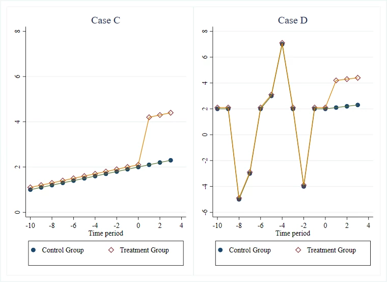
The event studies for the two settings will look remarkably similar: reasonable pre-trends followed by a treatment effect. However, the latter is intuitively more credible than the former because the two groups are getting hit by shocks in the pre-period and responding in similar ways, which suggests to us that they are quite similar, and therefore the blue line is a credible counterfactual for the yellow one.

A flat or linear pre-trend is “smooth.” Many potential control units might match a smooth trend purely by chance (spurious correlation). Conversely, a trend that is “long and squiggly”—volatile, non-linear, and idiosyncratic—acts as a unique fingerprint. If a control unit tracks a treated unit’s complex volatility perfectly, it is statistically improbable that this is a coincidence. This intuitively makes it more credible that parallel trends.

We can move this intuition from a “visual check” to a rigorous adversarial framework using placebo testing and distributional embeddings.

The Intuition: Specificity vs. Generic Trends

The core claim is that “squiggly” data provides the uniqueness of the matched unit for counterfactual construction.

• Smooth Data (Low Volatility): If the outcome is roughly linear, the space of potential controls that satisfy the “parallel trends” check is large. The “true” control is indistinguishable from random noise or other spurious trends.
• Squiggly Data (High Volatility): If the outcome is driven by complex common shocks, the space of valid controls shrinks. Only a unit experiencing the exact same structural shocks will yield a low pre-treatment fit error.

Formalization Sketch

We can formalize this using the framework of Fisherian Randomization Inference applied to the Pre-treatment Mean Squared Prediction Error (RMSPE), a technique popularized by the Synthetic Control literature but equally applicable here.

1. The Setup

Let $Y_{it}$ be the outcome for unit $i$ at time $t$. A single unit is treated at time $T_0+1$.

• $i=0$: Treated unit.
• $i\in \{1,\dots ,N\}$: Pool of potential control units.
• $t\in \{1,\dots ,T_0\}$: Pre-treatment period.

We assume the data generating process for the outcome involves a shared latent factor ${\lambda }_t$:

$$Y_{it}={\alpha }_i+{\gamma }_i{\lambda }_t+{\epsilon }_{it}$$

Parallel trends hold strictly if the factor loadings are identical (${\gamma }_0={\gamma }_j$). This structure underpins many modern panel methods (Synthetic Control, Synthetic Diff-in-Diff etc): ultiple $\gamma$s are permitted - one either explicitly fits this structure (e.g. via a factor model - Generalized Synthetic Control, or Matrix Completion), or implicitly (least squares with ridge - SC + SDID).

2. The Adversarial Metric (RMSPE)

We define a loss function $L$ representing the “parallel trends gap” in the pre-period. A standard choice is the Root Mean Squared Prediction Error after subtracting off pre-treatment means (to account for unit fixed effects ${\alpha }_i$ - elsewhere McKenzie and others have argued that level differences make parallel trends less plausible, which is intuitively plausible but a separate problem):

$$J_i=\sqrt{\frac{1}{T_0}\sum _{t=1}^{T_0}{\left((Y_{0t}-{\bar{Y}}_0)-(Y_{it}-{\bar{Y}}_i)\right)}^2}$$

Where $J_i$ measures how well unit $i$ mimics the shape of the treated unit $0$.

3. The Test: Permutation Inference

We wish to test the null hypothesis $H_0$ that unit $i$ is exchangeable with the treated unit regarding the trend. We compute the rank of the “True Control” (or our proposed control group) against the distribution of all placebo controls $k\in \{2,\dots ,N\}$.

$$p\text{-value}=\frac{1}{N}\sum _{k=1}^N\mathbb{I}(J_k\le J_{\text{proposed}})$$

4. Why “Squiggly” Wins

• In the Smooth Case: $\text{Var}({\lambda }_t)\approx 0$. The term ${\gamma }_i{\lambda }_t$ is dominated by noise ${\epsilon }_{it}$. $J_i$ is determined largely by random noise. The true control ($i=1$) has no distinct advantage over random placebos ($i=k$).

  • Result: Uniform distribution of ranks. High $p$-value.

• In the Squiggly Case: $\text{Var}({\lambda }_t)\gg \text{Var}(\epsilon )$. The term ${\gamma }_i{\lambda }_t$ dominates. If unit $1$ shares the factor (${\gamma }_1\approx {\gamma }_0$) and unit $k$ does not, then $J_1\to 0$ while $J_k\gg 0$.
  • Result: The true control is strictly separated from the distribution. $p\to 1/N$.

Empirical Demonstration

We simulated this logic using two scenarios: a linear trend (“Smooth”) and a volatile random walk (“Squiggly”). There is always one `true’ correct control, and if we were to identify that, our estimates would have the lowest bias.

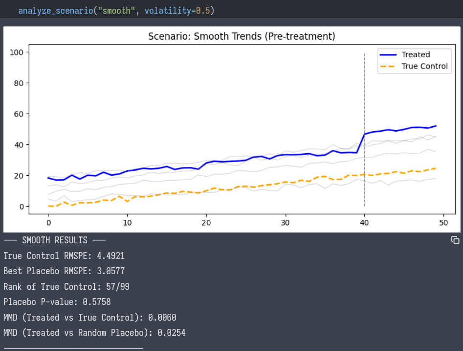
Scenario A: The Smooth Trend

• Visual: The lines look parallel. Standard event studies would likely pass.
• Adversarial Test:
  • True Control RMSPE: 4.49
  • Best Placebo RMSPE: 3.05 (A random unit matched better than the true control!)
  • Rank: 57 / 99
  • P-value: 0.57
• Conclusion: We cannot rigorously claim specific parallel trends. The “match” is statistically indistinguishable from noise.

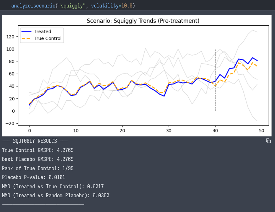
Scenario B: The Squiggly Trend

• Visual: The treated unit moves erratically. The control unit matches every move.
• Adversarial Test:
  • True Control RMSPE: 4.27
  • Best Placebo RMSPE: 4.27. The true control is the minimizer of the RMSPE metric.
  • Rank: 1 / 99
  • P-value: 0.01
• Conclusion: The match is unique. The probability of a random unit matching this complex “squiggle” by chance is effectively zero.

Distributional Testing (Kernel MMD)

Beyond RMSPE (which measures point-wise distance), we could consider using Maximum Mean Discrepancy (MMD) to test if the changes in outcomes ($\Delta Y_t$) come from the same distribution.

Using this insight in practice

In reality, we don’t know the true control, so this placebo isn’t yet unusable. However, we can make this useful if we move the goalposts a bit: Instead of comparing “Treated vs. Unit 1,” we could compare “How well can we fit the Treated unit?” vs. “How well can we fit any other unit?”

1. The Donor Pool: Let $J$ be the set of all untreated units.
2. Estimate the Treated Counterfactual: Use an algorithm (OLS, Lasso, Synthetic Control constraints) to find the weighted combination of units in $J$ that minimizes the pre-treatment RMSPE for the treated unit.
   • Let this error be $E_{treated}$.
3. Estimate Placebo Counterfactuals: For every unit $j$ in the donor pool:
   • Pretend $j$ is the treated unit.
   • Use the remaining units ($J\setminus j$) to construct a synthetic control for $j$.
   • Calculate the minimized pre-treatment RMSPE, $E_j$.
4. The Ratio: Compare $E_{treated}$ against the distribution of $\{E_j\}$.

• Smooth Case: Trends are generic. I can likely construct a very good synthetic match for any unit in the dataset using a linear combination of other units.

  • Result: $E_{treated}\approx E_{placebo}$. The treated unit is not special.

• Squiggly Case: Trends are specific fingerprints.

  • I can only construct a good match for the Treated unit IF the donor pool contains units that share its specific structural shocks.
  • However, if I try to construct a match for a random Placebo unit (which has its own idiosyncratic random walk), the donor pool may not span that specific path.
  • Result: $E_{treated}\ll E_{placebo}$. The treated unit stands out as uniquely “matchable,” implying a structural relationship rather than a spurious one.

By comparing the fit of the treated unit against the distribution of fits for all other units, we rigorously quantify the “long and squiggly” intuition without needing to know who the true controls are. We only need to assume that if good control matches, they will manifest as a uniquely tight fit compared to spurious matches.

This is the critical “fatal flaw” of the adversarial mindset if applied universally. You have correctly identified that this test is effectively a test for Hidden Structure, which is only desirable when you don’t have Random Assignment.

Coda: The RCT Paradox and When to Stop

Consider an ideal RCT. Treatment is assigned randomly. By definition, the treated unit is exchangeable with any control unit.

• If we run the Placebo Fit Test on an RCT, the treated unit should look exactly like the others.
• Its pre-trend fit (RMSPE) will be “average” compared to the donor pool.
• Its rank will be roughly $N/2$.

If you rigorously demand “specificity” (a rank of $1/N$) in an RCT, you will reject valid experiments. You will look at a perfectly randomized treatment group and say, “This isn’t credible because the control group matches the treatment group too easily.”

This reveals the fundamental difference in the burden of proof between experimental and observational designs:

1. In an RCT (The “Smooth” Ideal):

   • Assumption: We know the assignment mechanism (randomization).
   • Goal: We want the treated unit to be generic. We want it to be effectively indistinguishable from the herd until the treatment hits.
   • Result: High “smoothness,” low specificity. This is a feature.

2. In Observational DiD (The “Squiggly” Requirement):

   • Assumption: We do not know the assignment mechanism. We fear that the treated unit was selected because of some unobserved factor.
   • Goal: We need to prove that we have found the rare control unit that shares this unobserved factor.
   • Result: High specificity, low “smoothness.” We need the match to be “hard” to achieve so that we can be confident it isn’t spurious.

The “Long and Squiggly” standard is a stress test for constructed counterfactuals.

• Use when you have used Synthetic Control, Matching, or Lasso to find a control group from a messy donor pool. If your match is the only one that fits the squiggles, you have identified a latent structure.
• Do not use it when a valid control group was gifted to you by randomization. In that world, “long and squiggly” is just noise, and “smooth” is an indicator of validity.

---

Appendix

code - prototyped by an LLM and iterated upon after.

import matplotlib.pyplot as plt
import numpy as np
import pandas as pd
from sklearn.metrics.pairwise import rbf_kernel
 
np.random.seed(42)
 
 
# 
def compute_mmd(x, y, sigma=1.0):
    """
    Computes Maximum Mean Discrepancy (MMD) between two sequence distributions.
    Here we compare the distribution of first-differences (changes) to check
    if the 'volatility profile' matches.
    """
    x = x.reshape(-1, 1)
    y = y.reshape(-1, 1)
 
    K_xx = rbf_kernel(x, x, gamma=1.0 / (2 * sigma**2))
    K_yy = rbf_kernel(y, y, gamma=1.0 / (2 * sigma**2))
    K_xy = rbf_kernel(x, y, gamma=1.0 / (2 * sigma**2))
 
    mmd = np.mean(K_xx) + np.mean(K_yy) - 2 * np.mean(K_xy)
    return mmd
 
 
# 
analyze_scenario("smooth", volatility=0.5)
analyze_scenario("squiggly", volatility=10.0)
 
# %%