Intermediate Earth Data Science Notes
In [1]:
# system
import os, sys, glob, re, itertools, collections
from pathlib import Path

# pyscience imports
import numpy as np
import pandas as pd
import statsmodels.api as sm
import statsmodels.formula.api as smf

# viz
import matplotlib.pyplot as plt
import seaborn as sns
from plotnine import *
# plt.style.use("seaborn-darkgrid")
sns.set(style="ticks", context="talk")
font = {'family' : 'IBM Plex Sans',
               'weight' : 'normal',
               'size'   : 10}
plt.rc('font', **font)


# geodata packages
import geopandas as gpd
import geoplot as gplt
import mapclassify as mc
import geoplot.crs as gcrs
import earthpy as et
import earthpy.plot as ep

# raster packages
import rasterio as rio
from rasterstats import zonal_stats

# show all output
from IPython.core.interactiveshell import InteractiveShell
InteractiveShell.ast_node_interactivity = 'all'
#%%
In [2]:
os.chdir(os.path.join(et.io.HOME, 'earth-analytics'))
In [5]:
# Set working directory
os.chdir(os.path.join(et.io.HOME, 'earth-analytics'))
In [4]:
# Download csv of temp (F) and precip (inches) in July 2018 for Boulder, CO
file_url = "https://ndownloader.figshare.com/files/12948515"
et.data.get_data(url=file_url)
Out[4]:
In [6]:
# Define relative path to file
file_path = os.path.join("data", "earthpy-downloads",
                         "july-2018-temperature-precip.csv")
Parse datetime on read
In [8]:
# Import file into pandas dataframe
boulder_july_2018 = pd.read_csv(file_path, parse_dates=['date'], index_col = ['date'])
boulder_july_2018.head()
Out[8]:
In [9]:
boulder_july_2018.info()
In [12]:
# Create figure and plot space
fig, ax = plt.subplots(figsize=(10, 10))

# Add x-axis and y-axis
ax.scatter(boulder_july_2018.index.values,
        boulder_july_2018['precip'],
        color='purple')

# Set title and labels for axes
ax.set(xlabel="Date",
       ylabel="Precipitation (inches)",
       title="Daily Total Precipitation\nBoulder, Colorado in July 2018")

plt.setp(ax.get_xticklabels(), rotation=90)
plt.show()
Out[12]:
Out[12]:
Out[12]:
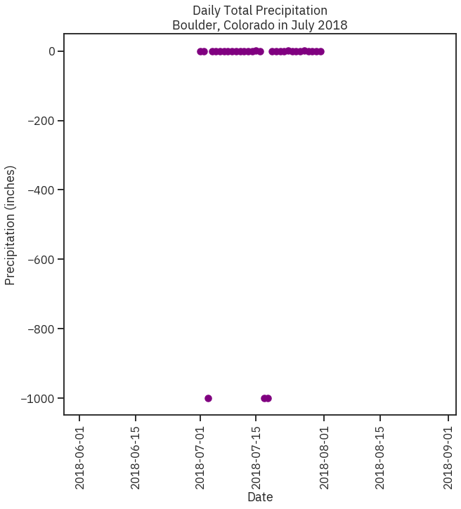
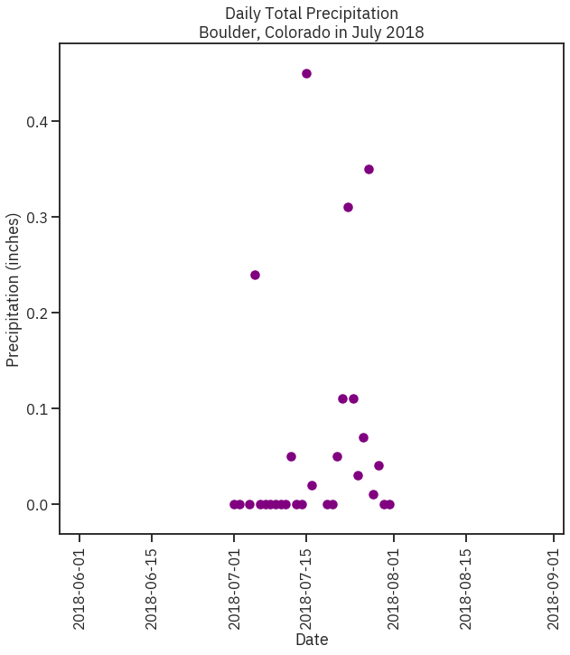
Read Missing values correctly
In [18]:
# Import file into pandas dataframe
boulder_july_2018 = pd.read_csv(file_path, parse_dates=['date'], index_col = ['date'])
boulder_july_2018.loc[boulder_july_2018.precip == -999, ['precip']] = None
boulder_july_2018.head()
Out[18]:
In [19]:
# Create figure and plot space
fig, ax = plt.subplots(figsize=(10, 10))

# Add x-axis and y-axis
ax.scatter(boulder_july_2018.index.values,
        boulder_july_2018['precip'],
        color='purple')

# Set title and labels for axes
ax.set(xlabel="Date",
       ylabel="Precipitation (inches)",
       title="Daily Total Precipitation\nBoulder, Colorado in July 2018")

plt.setp(ax.get_xticklabels(), rotation=90)
plt.show()
Out[19]:
Out[19]:
Out[19]:
TS Slices
In [20]:
# Download the data
data = et.data.get_data('colorado-flood')
# Set working directory
os.chdir(os.path.join(et.io.HOME, 'earth-analytics'))

# Define relative path to file with daily precip total
file_path = os.path.join("data", "colorado-flood",
                         "precipitation",
                         "805325-precip-dailysum-2003-2013.csv")
In [22]:
# Import data using datetime and no data value
boulder_precip_2003_2013 = pd.read_csv(file_path,
                                       parse_dates=['DATE'],
                                       index_col= ['DATE'],
                                       na_values=['999.99'])

boulder_precip_2003_2013.head()
boulder_precip_2003_2013.info()
Out[22]:
In [23]:
boulder_precip_2003_2013.describe()
Out[23]:
row-index slices w time
In [25]:
# select 2013 data - datetime index is magic
boulder_precip_2003_2013['2013'].head()
Out[25]:
In [26]:
# Select all December data - view first few rows
boulder_precip_2003_2013[boulder_precip_2003_2013.index.month == 12].head()
Out[26]:
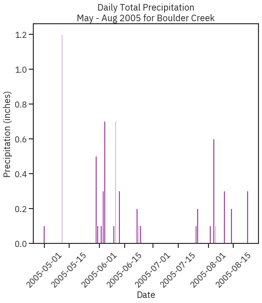
Range slice
In [27]:
# Subset data to May-Aug 2005
precip_may_aug_2005 = boulder_precip_2003_2013['2005-05-01':'2005-08-31']
precip_may_aug_2005.head()
Out[27]:
In [28]:
# Create figure and plot space
fig, ax = plt.subplots(figsize=(8, 8))

# Add x-axis and y-axis
ax.bar(precip_may_aug_2005.index.values,
       precip_may_aug_2005['DAILY_PRECIP'],
       color='purple')

# Set title and labels for axes
ax.set(xlabel="Date",
       ylabel="Precipitation (inches)",
       title="Daily Total Precipitation\nMay - Aug 2005 for Boulder Creek")

# Rotate tick marks on x-axis
plt.setp(ax.get_xticklabels(), rotation=45)

plt.show()
Out[28]:
Out[28]:
Out[28]:
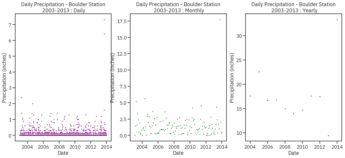
Resampling/Aggregating
In [7]:
# Define relative path to file with hourly precip
file_path = os.path.join("data", "colorado-flood",
                         "precipitation",
                         "805325-precip-daily-2003-2013.csv")

# Import data using datetime and no data value
precip_2003_2013_hourly = pd.read_csv(file_path,
                                      parse_dates=['DATE'],
                                      index_col=['DATE'],
                                      na_values=['999.99'])

# View first few rows
precip_2003_2013_hourly.head()
precip_2003_2013_hourly.info()
precip_2003_2013_hourly.describe()
Out[7]:
Out[7]:
In [8]:
# hourly index
precip_2003_2013_hourly.index
Out[8]:
In [26]:
# Resample to daily precip sum and save as new dataframe
precip_2003_2013_daily = precip_2003_2013_hourly.resample('D').sum()
# Resample to monthly precip sum and save as new dataframe
precip_2003_2013_monthly = precip_2003_2013_daily.resample('M').sum()
# Resample to yearly precip sum and save as new dataframe
precip_2003_2013_yearly = precip_2003_2013_hourly.resample('Y').sum()
In [28]:
# Create figure and plot space
fig, ax = plt.subplots(1, 3, figsize=(20, 8))


# Add x-axis and y-axis
ax[0].scatter(precip_2003_2013_daily.index.values,
           precip_2003_2013_daily['HPCP'], s = 2,
           color='purple')
# Set title and labels for axes
ax[0].set(xlabel="Date",
       ylabel="Precipitation (inches)",
       title="Daily Precipitation - Boulder Station\n 2003-2013 : Daily")

# Add x-axis and y-axis
ax[1].scatter(precip_2003_2013_monthly.index.values,
           precip_2003_2013_monthly['HPCP'], s = 2,
           color='green')
# Set title and labels for axes
ax[1].set(xlabel="Date",
       ylabel="Precipitation (inches)",
       title="Daily Precipitation - Boulder Station\n 2003-2013 : Monthly")
# Add x-axis and y-axis
ax[2].scatter(precip_2003_2013_yearly.index.values,
           precip_2003_2013_yearly['HPCP'], s = 2,
           color='blue')
# Set title and labels for axes
ax[2].set(xlabel="Date",
       ylabel="Precipitation (inches)",
       title="Daily Precipitation - Boulder Station\n 2003-2013 : Yearly")
Out[28]:
Out[28]:
Out[28]:
Out[28]:
Out[28]:
Out[28]:
Date Formats for plots
In [37]:
import matplotlib.dates as mdates
from matplotlib.dates import DateFormatter
In [29]:
# Define relative path to file with daily precip
file_path = os.path.join("data", "colorado-flood",
"precipitation",
"805325-precip-dailysum-2003-2013.csv")
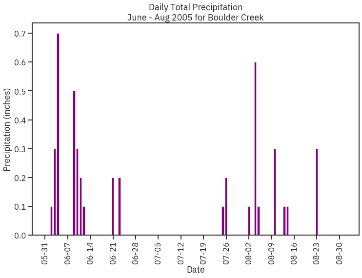
precip_june_aug_2005 = precip_2003_2013_daily['2005-06-01':'2005-08-31']
precip_june_aug_2005.head()
Out[29]:
In [41]:
# Create figure and plot space
fig, ax = plt.subplots(figsize=(12, 8))

# Add x-axis and y-axis
ax.bar(precip_june_aug_2005.index.values,
       precip_june_aug_2005['HPCP'],
       color='purple')

# Set title and labels for axes
ax.set(xlabel="Date",
       ylabel="Precipitation (inches)",
       title="Daily Total Precipitation\nJune - Aug 2005 for Boulder Creek")

date_form = DateFormatter("%m-%d")
ax.xaxis.set_major_formatter(date_form)

# Ensure a major tick for each week using (interval=1)
ax.xaxis.set_major_locator(mdates.WeekdayLocator(interval=1))
plt.setp(ax.get_xticklabels(), rotation=90)

plt.show()
Out[41]:
Out[41]:
Out[41]:
In [2]:
# Get data and set working directory
data = et.data.get_data('spatial-vector-lidar')
# Define path to file
plot_centroid_path = os.path.join("data", "spatial-vector-lidar",
"california", "neon-sjer-site",
"vector_data", "SJER_plot_centroids.shp")
# Import shapefile using geopandas
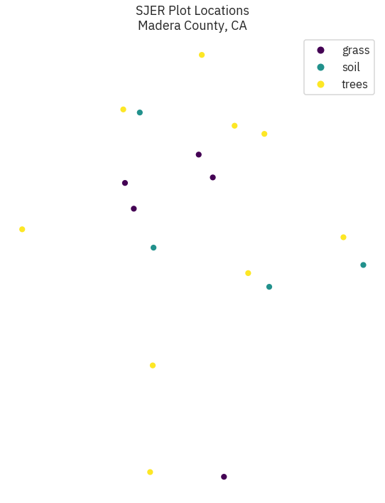
sjer_plot_locations = gpd.read_file(plot_centroid_path)
In [10]:
# View top 6 rows of attribute table
sjer_plot_locations.head(6)
Out[10]:
In [9]:
f, ax = plt.subplots(figsize = (10, 12))
sjer_plot_locations.plot(column = 'plot_type', categorical = True, legend = True,
                         markersize = 45, cmap = "viridis", ax = ax)
ax.set_title('SJER Plot Locations\nMadera County, CA')
ax.set_axis_off()
# f.savefig(out/'location.pdf')
Out[9]:
Out[9]:
Projections/CRS
In [29]:
from shapely.geometry import Point, Polygon
from matplotlib.ticker import ScalarFormatter
In [30]:
sjer_plot_locations.crs
sjer_plot_locations.total_bounds
Out[30]:
Out[30]:
In [31]:
# Import world boundary shapefile
worldBound_path = os.path.join("data", "spatial-vector-lidar", "global",
                               "ne_110m_land", "ne_110m_land.shp")
worldBound = gpd.read_file(worldBound_path)
worldBound.crs
Out[31]:
In [32]:
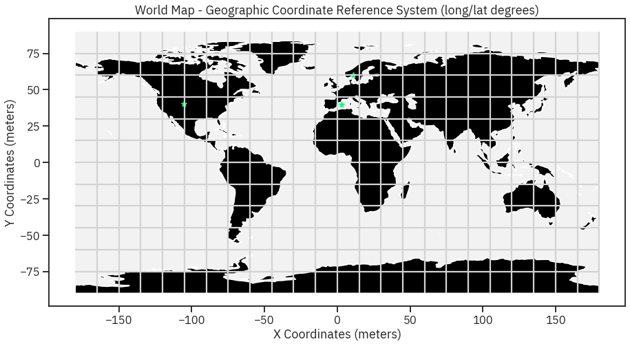
# Create numpy array of x,y point locations
add_points = np.array([[-105.2519,   40.0274],
                       [  10.75  ,   59.95  ],
                       [   2.9833,   39.6167]])

# Turn points into list of x,y shapely points
city_locations = [Point(xy) for xy in add_points]
# Create geodataframe using the points
city_locations = gpd.GeoDataFrame(city_locations,
                                  columns=['geometry'],
                                  crs=worldBound.crs)
In [34]:
# Import graticule & world bounding box shapefile data
graticule_path = os.path.join("data", "spatial-vector-lidar", "global",
                              "ne_110m_graticules_all", "ne_110m_graticules_15.shp")
graticule = gpd.read_file(graticule_path)

bbox_path = os.path.join("data", "spatial-vector-lidar", "global",
                         "ne_110m_graticules_all", "ne_110m_wgs84_bounding_box.shp")
bbox = gpd.read_file(bbox_path)

# Create map axis object
fig, ax = plt.subplots(1, 1, figsize=(15, 8))
# Add bounding box and graticule layers
bbox.plot(ax=ax, alpha=.1, color='grey')
graticule.plot(ax=ax, color='lightgrey')
worldBound.plot(ax=ax, color='black')

# Add points to plot
city_locations.plot(ax=ax,
                    markersize=60,
                    color='springgreen',
                    marker='*')
# Add title and axes labels
ax.set(title="World Map - Geographic Coordinate Reference System (long/lat degrees)",
       xlabel="X Coordinates (meters)",
       ylabel="Y Coordinates (meters)");
Robinson
In [35]:
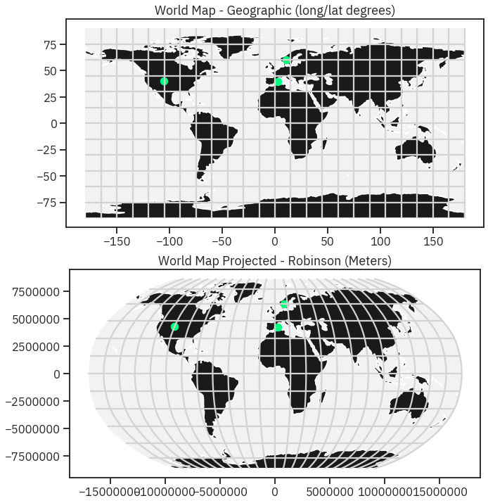
# Reproject the data
worldBound_robin = worldBound.to_crs('+proj=robin')
graticule_robin = graticule.to_crs('+proj=robin')
city_locations_robin = city_locations.to_crs(worldBound_robin.crs)
bbox_robinson = bbox.to_crs('+proj=robin')
In [36]:
# Setup plot with 2 "rows" one for each map and one column
fig, (ax0, ax1) = plt.subplots(2, 1, figsize=(13, 12))

# First plot
bbox.plot(ax=ax0,
          alpha=.1,
          color='grey')

graticule.plot(ax=ax0,
               color='lightgrey')

worldBound.plot(ax=ax0,
                color='k')

city_locations.plot(ax=ax0,
                    markersize=100,
                    color='springgreen')

ax0.set(title="World Map - Geographic (long/lat degrees)")

# Second plot
bbox_robinson.plot(ax=ax1,
                   alpha=.1,
                   color='grey')

graticule_robin.plot(ax=ax1,
                        color='lightgrey')

worldBound_robin.plot(ax=ax1,
                      color='k')

city_locations_robin.plot(ax=ax1,
                          markersize=100,
                          color='springgreen')

ax1.set(title="World Map Projected - Robinson (Meters)")

for axis in [ax1.xaxis, ax1.yaxis]:
    formatter = ScalarFormatter()
    formatter.set_scientific(False)
    axis.set_major_formatter(formatter)
Out[36]:
Out[36]:
Out[36]:
Out[36]:
Out[36]:
Out[36]:
Out[36]:
Out[36]:
Out[36]:
Out[36]:
Reprojecting
In [37]:
# Import the data
sjer_roads_path = os.path.join("data", "spatial-vector-lidar", "california",
                               "madera-county-roads", "tl_2013_06039_roads.shp")
sjer_roads = gpd.read_file(sjer_roads_path)

# aoi stands for area of interest
sjer_aoi_path = os.path.join("data", "spatial-vector-lidar", "california",
                             "neon-sjer-site", "vector_data", "SJER_crop.shp")
sjer_aoi = gpd.read_file(sjer_aoi_path)
In [38]:
# View the Coordinate Reference System of both layers
sjer_roads.crs
sjer_aoi.crs
Out[38]:
Out[38]:
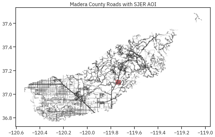
In [39]:
# Reproject the aoi to match the roads layer
sjer_aoi_wgs84  = sjer_aoi.to_crs(epsg=4269)

# Plot the data
fig, ax = plt.subplots(figsize=(12, 8))

sjer_roads.plot(cmap='Greys', ax=ax, alpha=.5)
sjer_aoi_wgs84.plot(ax=ax, markersize=10, color='r')

ax.set_title("Madera County Roads with SJER AOI");
Census
In [40]:
# Import data into geopandas dataframe
state_boundary_us_path = os.path.join("data", "spatial-vector-lidar",
                                      "usa", "usa-states-census-2014.shp")
state_boundary_us = gpd.read_file(state_boundary_us_path)

# View data structure
type(state_boundary_us)
state_boundary_us.crs
Out[40]:
Out[40]:
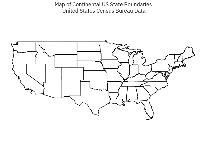
In [41]:
# Plot the data
fig, ax = plt.subplots(figsize = (12,8))
state_boundary_us.plot(ax = ax, facecolor = 'white', edgecolor = 'black')

# Add title to map
ax.set(title="Map of Continental US State Boundaries\n United States Census Bureau Data")

# Turn off the axis
plt.axis('equal')
ax.set_axis_off()

plt.show()
Out[41]:
Out[41]:
Out[41]:
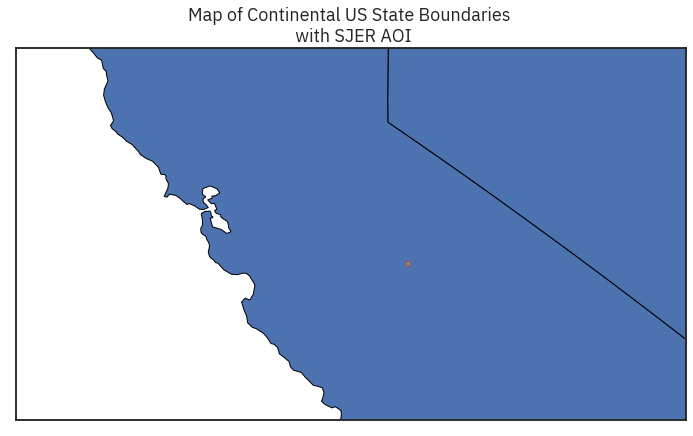
In [43]:
# Zoom in on just the area
fig, ax = plt.subplots(figsize = (12,8))

state_boundary_us.plot(ax = ax,
                      linewidth=1,
                      edgecolor="black")

sjer_aoi_wgs84.plot(ax=ax,
                    color='springgreen',
                   edgecolor = "r")

ax.set(title="Map of Continental US State Boundaries \n with SJER AOI")
ax.set(xlim=[-125, -116], ylim=[35, 40])

# Turn off axis
ax.set(xticks = [], yticks = []);
Clipping
Points in Extent
In [3]:
# Import all of your data at the top of your notebook to keep things organized.
country_boundary_us_path = os.path.join("data", "spatial-vector-lidar",
                                        "usa", "usa-boundary-dissolved.shp")
country_boundary_us = gpd.read_file(country_boundary_us_path)

state_boundary_us_path = os.path.join("data", "spatial-vector-lidar",
                                      "usa", "usa-states-census-2014.shp")
state_boundary_us = gpd.read_file(state_boundary_us_path)

pop_places_path = os.path.join("data", "spatial-vector-lidar", "global",
                               "ne_110m_populated_places_simple", "ne_110m_populated_places_simple.shp")
pop_places = gpd.read_file(pop_places_path)

# Are the data all in the same crs?
print("country_boundary_us", country_boundary_us.crs)
print("state_boundary_us", state_boundary_us.crs)
print("pop_places", pop_places.crs)
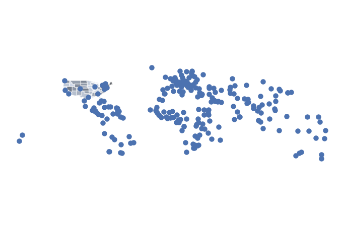
In [4]:
# Plot the data
fig, ax = plt.subplots(figsize=(12, 8))

country_boundary_us.plot(alpha=.5,
                         ax=ax)

state_boundary_us.plot(cmap='Greys',
                       ax=ax,
                       alpha=.5)
pop_places.plot(ax=ax)

plt.axis('equal')
ax.set_axis_off()
plt.show()
Out[4]:
Out[4]:
Out[4]:
Out[4]:
In [5]:
# Clip the data using GeoPandas clip
points_clip = gpd.clip(pop_places, country_boundary_us)

# View the first 6 rows and a few select columns
points_clip[['name', 'geometry', 'scalerank', 'natscale', ]].head()
Out[5]:
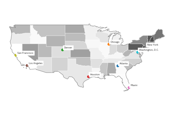
In [6]:
# Plot the data
fig, ax = plt.subplots(figsize=(12, 8))

country_boundary_us.plot(alpha=1,
                         color="white",
                         edgecolor="black",
                         ax=ax)

state_boundary_us.plot(cmap='Greys',
                       ax=ax,
                       alpha=.5)

points_clip.plot(ax=ax,
                 column='name')
ax.set_axis_off()
plt.axis('equal')

# Label each point - note this is just shown here optionally but is not required for your homework
points_clip.apply(lambda x: ax.annotate(s=x['name'],
                                        xy=x.geometry.coords[0],
                                        xytext=(6, 6), textcoords="offset points",
                                        backgroundcolor="white"),
                  axis=1)
plt.show()
Out[6]:
Out[6]:
Out[6]:
Out[6]:
Out[6]:
Line or Polygon in Extent
In [7]:
# Open the roads layer
ne_roads_path = os.path.join("data", "spatial-vector-lidar", "global",
                             "ne_10m_roads", "ne_10m_roads.shp")
ne_roads = gpd.read_file(ne_roads_path)

# Are both layers in the same CRS?
if (ne_roads.crs == country_boundary_us.crs):
    print("Both layers are in the same crs!",
          ne_roads.crs, country_boundary_us.crs)
In [8]:
# Simplify the geometry of the clip extent for faster processing
# Use this with caution as it modifies your data.
country_boundary_us_sim = country_boundary_us.simplify(
    .2, preserve_topology=True)
In [9]:
# Clip data
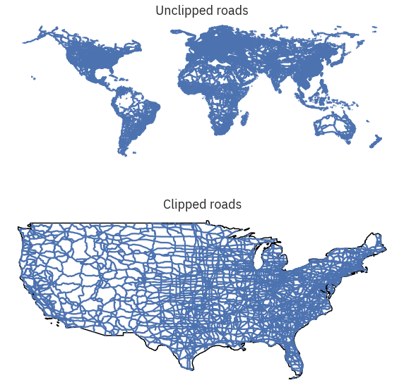
ne_roads_clip = gpd.clip(ne_roads, country_boundary_us_sim)
# Ignore missing/empty geometries
ne_roads_clip = ne_roads_clip[~ne_roads_clip.is_empty]
print("The clipped data have fewer line objects (represented by rows):",
ne_roads_clip.shape, ne_roads.shape)
In [11]:
fig, (ax1, ax2) = plt.subplots(2, 1, figsize=(10, 10))

ne_roads.plot(ax=ax1)
country_boundary_us.plot(alpha=1,
                         color="white",
                         edgecolor="black",
                         ax=ax2)
ne_roads_clip.plot(ax=ax2)

ax1.set_title("Unclipped roads")
ax2.set_title("Clipped roads")

ax1.set_axis_off()
ax2.set_axis_off()

plt.axis('equal')
plt.show()
Out[11]:
Out[11]:
Out[11]:
Out[11]:
Out[11]:
Out[11]:
Other Spatial Operations
Simplifying polygons
In [12]:
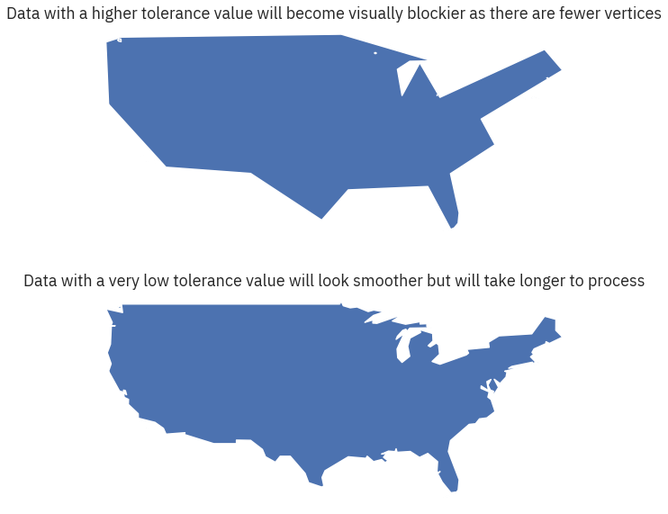
fig, (ax1, ax2) = plt.subplots(2, 1, figsize=(10, 10))

# Set a larger tolerance yields a blockier polygon
country_boundary_us.simplify(2, preserve_topology=True).plot(ax=ax1)

# Set  a larger tolerance yields a blockier polygon
country_boundary_us.simplify(.2, preserve_topology=True).plot(ax=ax2)

ax1.set_title( "Data with a higher tolerance value will become visually blockier as there are fewer vertices")
ax2.set_title( "Data with a very low tolerance value will look smoother but will take longer to process")

ax1.set_axis_off()
ax2.set_axis_off()
plt.show()
Out[12]:
Out[12]:
Out[12]:
Out[12]:
Dissolving Polygons
In [13]:
state_boundary = state_boundary_us[['LSAD', 'geometry']]
cont_usa = state_boundary.dissolve(by='LSAD')

# View the resulting geodataframe
cont_usa
Out[13]:
In [14]:
# Select the columns that you wish to retain in the data
state_boundary = state_boundary_us[['region', 'geometry', 'ALAND', 'AWATER']]

# Then summarize the quantative columns by 'sum'
regions_agg = state_boundary.dissolve(by='region', aggfunc='sum')
regions_agg
Out[14]:
In [24]:
mc.Quantiles(regions_agg.ALAND, k=5).bins
# mc.Quantiles(regions_agg.AWATER, k=5)
Out[24]:
Spatial Joins
In [25]:
# Roads within region
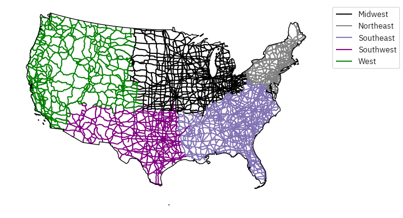
roads_region = gpd.sjoin(ne_roads_clip,
regions_agg,
how="inner",
op='intersects')
# Notice once you have joins the data - you have attributes
# from the regions_object (i.e. the region) attached to each road feature
roads_region[["featurecla", "index_right", "ALAND"]].head()
Out[25]:
In [27]:
# Reproject to Albers for plotting
country_albers = cont_usa.to_crs({'init': 'epsg:5070'})
roads_albers = roads_region.to_crs({'init': 'epsg:5070'})

# First, create a dictionary with the attributes of each legend item
road_attrs = {'Midwest': ['black'],
              'Northeast': ['grey'],
              'Southeast': ['m'],
              'Southwest': ['purple'],
              'West': ['green']}

# Plot the data
fig, ax = plt.subplots(figsize=(12, 8))

regions_agg.plot(edgecolor="black",
                 ax=ax)
country_albers.plot(alpha=1,
                    facecolor="none",
                    edgecolor="black",
                    zorder=10,
                    ax=ax)

for ctype, data in roads_albers.groupby('index_right'):
    data.plot(color=road_attrs[ctype][0],
              label=ctype,
              ax=ax)

# This approach works to place the legend when you have defined labels
plt.legend(bbox_to_anchor=(1.0, 1), loc=2)
ax.set_axis_off()
plt.axis('equal')
plt.show()
Out[27]:
Out[27]:
Out[27]:
Out[27]:
Out[27]:
Out[27]:
Out[27]:
Out[27]:
Out[27]:
Calculate Line Segment Length
In [29]:
# Turn off scientific notation
pd.options.display.float_format = '{:.4f}'.format

# Calculate the total length of road
road_albers_length = roads_albers[['index_right', 'length_km']]

# Sum existing columns
# roads_albers.groupby('index_right').sum()

roads_albers['rdlength'] = roads_albers.length
sub = roads_albers[['rdlength', 'index_right']].groupby('index_right').sum()
sub
Out[29]:
Rasters
In [50]:
from shapely.geometry import Polygon, mapping, box
import rasterio as rio
from rasterio.mask import mask
from rasterio.plot import show
import pprint
Metadata
In [52]:
# Define relative path to file
lidar_dem_path = os.path.join("data", "colorado-flood", "spatial",
                              "boulder-leehill-rd", "pre-flood", "lidar",
                              "pre_DTM.tif")

# View crs of raster imported with rasterio
with rio.open(lidar_dem_path) as src:
    print(src.crs)
    print(src.bounds)
    print(src.res)
    print("---")
    pprint.pprint(src.meta)
In [33]:
# Each key of the dictionary is an EPSG code
print(list(et.epsg.keys())[:10])

# You can convert to proj4 like so:
proj4 = et.epsg['32613']
print(proj4)
crs_proj4 = rio.crs.CRS.from_string(proj4)
crs_proj4
Out[33]:
Display
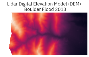
In [36]:
# Open raster data
lidar_dem = rio.open(lidar_dem_path)
# Plot the dem using raster.io
fig, ax = plt.subplots(figsize = (8,3))

show(lidar_dem,
     title="Lidar Digital Elevation Model (DEM) \n Boulder Flood 2013",
     ax=ax)

ax.set_axis_off()
lidar_dem.close()
Out[36]:
In [54]:
with rio.open(lidar_dem_path) as src:
    # Convert / read the data into a numpy array
    # masked = True turns `nodata` values to nan
    lidar_dem_im = src.read(1, masked=True)
    lidar_dem_mask = src.dataset_mask()
    # Create a spatial extent object using rio.plot.plotting
    spatial_extent = rio.plot.plotting_extent(src)

print("object shape:", lidar_dem_im.shape)
print("object type:", type(lidar_dem_im))
Mask
In [55]:
lidar_dem_mask
Out[55]:
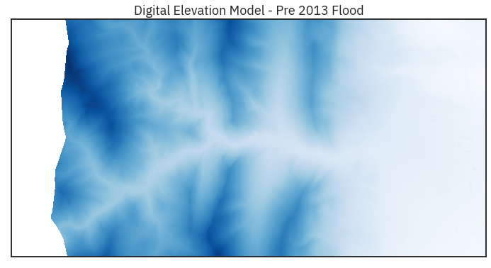
In [42]:
ep.plot_bands(lidar_dem_im,
              cmap='Blues',
              extent=spatial_extent,
              title="Digital Elevation Model - Pre 2013 Flood",
              cbar=False)
plt.show()
Out[42]:
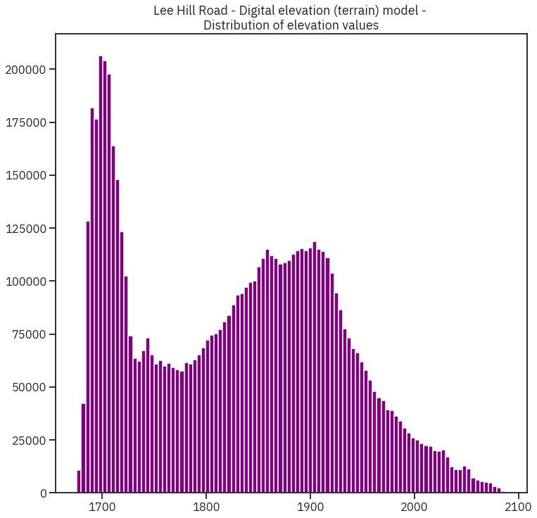
In [43]:
#### Plot histogram
ep.hist(lidar_dem_im[~lidar_dem_im.mask].ravel(),
        bins=100,
        title="Lee Hill Road - Digital elevation (terrain) model - \nDistribution of elevation values")
plt.show()
Out[43]:
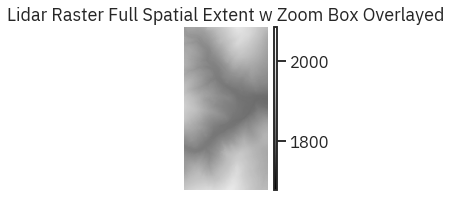
In [48]:
### Zoom in
# Define a spatial extent that is "smaller"
# minx, miny, maxx, maxy, ccw=True
zoomed_extent = [472500, 4434000, 473030, 4435030]
zoom_ext_gdf = gpd.GeoDataFrame()
zoom_ext_gdf.loc[0, 'geometry'] = box(*zoomed_extent)
fig, ax = plt.subplots(figsize=(8, 3))

ep.plot_bands(lidar_dem_im,
              extent=spatial_extent,
              title="Lidar Raster Full Spatial Extent w Zoom Box Overlayed",
              ax=ax,
              scale=False)

# Set x and y limits of the plot
ax.set_xlim(zoomed_extent[0], zoomed_extent[2])
ax.set_ylim(zoomed_extent[1], zoomed_extent[3])


ax.set_axis_off()
Out[48]:
Out[48]:
Out[48]:
Raster Processing
In [57]:
from rasterio.plot import plotting_extent
Subtract Arrays
In [58]:
# Define relative path to file
lidar_dem_path = os.path.join("data", "colorado-flood", "spatial",
                              "boulder-leehill-rd", "pre-flood", "lidar",
                              "pre_DTM.tif")

# Open raster data
with rio.open(lidar_dem_path) as lidar_dem:
    lidar_dem_im = lidar_dem.read(1, masked=True)
    # Get bounds for plotting
    bounds = plotting_extent(lidar_dem)

# Define relative path to file
lidar_dsm_path = os.path.join("data", "colorado-flood", "spatial",
                              "boulder-leehill-rd", "pre-flood", "lidar",
                              "pre_DSM.tif")

with rio.open(lidar_dsm_path) as lidar_dsm:
    lidar_dsm_im = lidar_dsm.read(1, masked=True)

# Are the bounds the same?
print("Is the spatial extent the same?",
      lidar_dem.bounds == lidar_dsm.bounds)

# Is the resolution the same ??
print("Is the resolution the same?",
      lidar_dem.res == lidar_dsm.res)
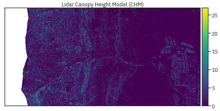
Tree height computation $$ CHM = DSM - DEM $$
In [59]:
# Calculate canopy height model
lidar_chm_im = lidar_dsm_im - lidar_dem_im
ep.plot_bands(lidar_chm_im,
              cmap='viridis',
              title="Lidar Canopy Height Model (CHM)",
              scale=False)
Out[59]:
In [60]:
ep.hist(lidar_chm_im,
        colors = 'purple',
        title="Histogram of CHM Values")
Out[60]:
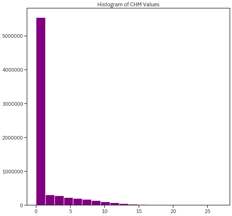
In [61]:
print('CHM minimum value: ', lidar_chm_im.min())
print('CHM max value: ', lidar_chm_im.max())
Export array as raster
In [64]:
lidar_chm_im
type(lidar_chm_im)
Out[64]:
Out[64]:
In [65]:
lidar_dem.meta
# Create dictionary copy
chm_meta = lidar_dem.meta.copy()
# Update the nodata value to be an easier to use number

# fill the masked pixels with a set no data value
nodatavalue = -999.0
lidar_chm_im_fi = np.ma.filled(lidar_chm_im, fill_value=nodatavalue)
lidar_chm_im_fi.min(), nodatavalue

chm_meta.update({'nodata': nodatavalue})
chm_meta
Out[65]:
Out[65]:
Out[65]:
In [67]:
%%time
out_path = "/home/alal/tmp/chm_export.tif"
with rio.open(out_path, 'w', **chm_meta) as outf:
    outf.write(lidar_chm_im_fi, 1)
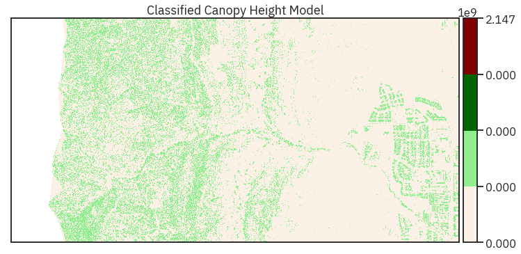
Reclassify raster (to account for skew)
In [70]:
# Define bins that you want, and then classify the data
class_bins = [lidar_chm_im.min(), 2, 7, 12, np.iinfo(np.int32).max]

# Classify the original image array, then unravel it again for plotting
lidar_chm_im_class = np.digitize(lidar_chm_im, class_bins)

# Note that you have an extra class in the data (0)
print(np.unique(lidar_chm_im_class))
In [71]:
lidar_chm_class_ma = np.ma.masked_where(lidar_chm_im_class == 0,
                                        lidar_chm_im_class,
                                        copy=True)
lidar_chm_class_ma
Out[71]:
In [73]:
from matplotlib.colors import ListedColormap, BoundaryNorm
In [74]:
# Plot newly classified and masked raster
# ep.plot_bands(lidar_chm_class_ma,
#               scale=False)
# Plot data using nicer colors
colors = ['linen', 'lightgreen', 'darkgreen', 'maroon']

cmap = ListedColormap(colors)
norm = BoundaryNorm(class_bins, len(colors))

ep.plot_bands(lidar_chm_class_ma,
              cmap=cmap,
              title="Classified Canopy Height Model",
              scale=False,
              norm=norm)
plt.show()
Out[74]:
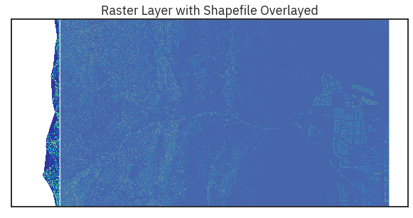
Clip raster
In [77]:
lidar= rio.open(lidar_dem_path)

aoi = os.path.join("data", "colorado-flood", "spatial",
                   "boulder-leehill-rd", "clip-extent.shp")

# Open crop extent (your study area extent boundary)
crop_extent = gpd.read_file(aoi)
print('crop extent crs: ', crop_extent.crs)
print('lidar crs: ', lidar.crs)
In [79]:
fig, ax = plt.subplots(figsize=(10, 8))

ep.plot_bands(lidar_chm_im, cmap='terrain',
              extent=plotting_extent(lidar),
              ax=ax,
              title="Raster Layer with Shapefile Overlayed",
              cbar=False)

crop_extent.plot(ax=ax, alpha=.8)
Out[79]:
Out[79]:
In [81]:
lidar_chm_crop, lidar_chm_crop_meta = et.spatial.crop_image(lidar,crop_extent)
lidar_chm_crop_affine = lidar_chm_crop_meta["transform"]
# Create spatial plotting extent for the cropped layer
lidar_chm_extent = plotting_extent(lidar_chm_crop[0], lidar_chm_crop_affine)
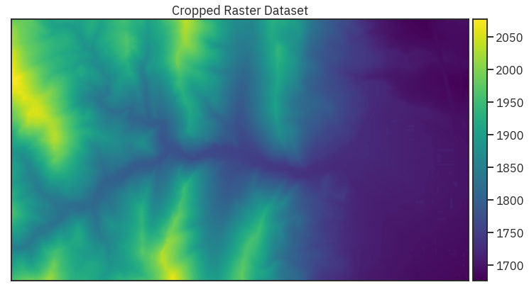
In [82]:
ep.plot_bands(lidar_chm_crop[0],
              extent=lidar_chm_extent,
              cmap='viridis',
              title="Cropped Raster Dataset",
              scale=False)
Out[82]:
Reproject Raster
In [85]:
from rasterio.warp import calculate_default_transform, reproject, Resampling
In [86]:
def reproject_et(inpath, outpath, new_crs):
    dst_crs = new_crs # CRS for web meractor

    with rio.open(inpath) as src:
        transform, width, height = calculate_default_transform(
            src.crs, dst_crs, src.width, src.height, *src.bounds)
        kwargs = src.meta.copy()
        kwargs.update({
            'crs': dst_crs,
            'transform': transform,
            'width': width,
            'height': height
        })

        with rio.open(outpath, 'w', **kwargs) as dst:
            for i in range(1, src.count + 1):
                reproject(
                    source=rio.band(src, i),
                    destination=rio.band(dst, i),
                    src_transform=src.transform,
                    src_crs=src.crs,
                    dst_transform=transform,
                    dst_crs=dst_crs,
                    resampling=Resampling.nearest)
In [90]:
inp = os.path.join("data", "colorado-flood", "spatial",
                                   "boulder-leehill-rd", "pre-flood", "lidar", "pre_DTM.tif")
out = "/home/alal/tmp/reprojected_lidar.tif"
reproject_et(inpath = inp,
             outpath = out,
             new_crs = 'EPSG:3857')
In [91]:
lidar_or   = rio.open(inp)
lidar_dem3 = rio.open(out)
pprint.pprint(lidar_or.meta)
pprint.pprint(lidar_dem3.meta)
lidar_or.close()
lidar_dem3.close()
Multispectral Rasters
In [9]:
import earthpy.spatial as es
LANDSAT

In [3]:
%%time
# Download data and set working directory
data = et.data.get_data('cold-springs-fire')
In [5]:
import glob
In [13]:
# Get list of all pre-cropped data and sort the data
path = os.path.join("data", "cold-springs-fire", "landsat_collect",
                    "LC080340322016072301T1-SC20180214145802", "crop")
all_landsat_post_bands =  glob.glob(path + '/*band*.tif')
all_landsat_post_bands.sort()
In [14]:
# Create an output array of all the landsat data stacked
landsat_post_fire_path = os.path.join("data", "cold-springs-fire",
                                      "outputs", "landsat_post_fire.tif")

# This will create a new stacked raster with all bands
land_stack, land_meta = es.stack(all_landsat_post_bands,
                                 landsat_post_fire_path)
In [15]:
with rio.open(landsat_post_fire_path) as src:
    landsat_post_fire = src.read()
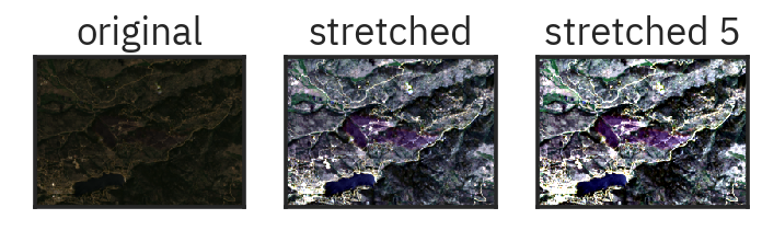
In [24]:
f, ax = plt.subplots(1, 3, dpi = 140)
ep.plot_rgb(landsat_post_fire,
            rgb=[3, 2, 1],
            title="original", ax = ax[0])
ep.plot_rgb(landsat_post_fire,
            rgb=[3, 2, 1], stretch=True, str_clip= 1,
            title="stretched", ax = ax[1])

ep.plot_rgb(landsat_post_fire,
            rgb=[3, 2, 1], stretch=True, str_clip= 5,
            title="stretched 5", ax = ax[2])
Out[24]:
Out[24]:
Out[24]:
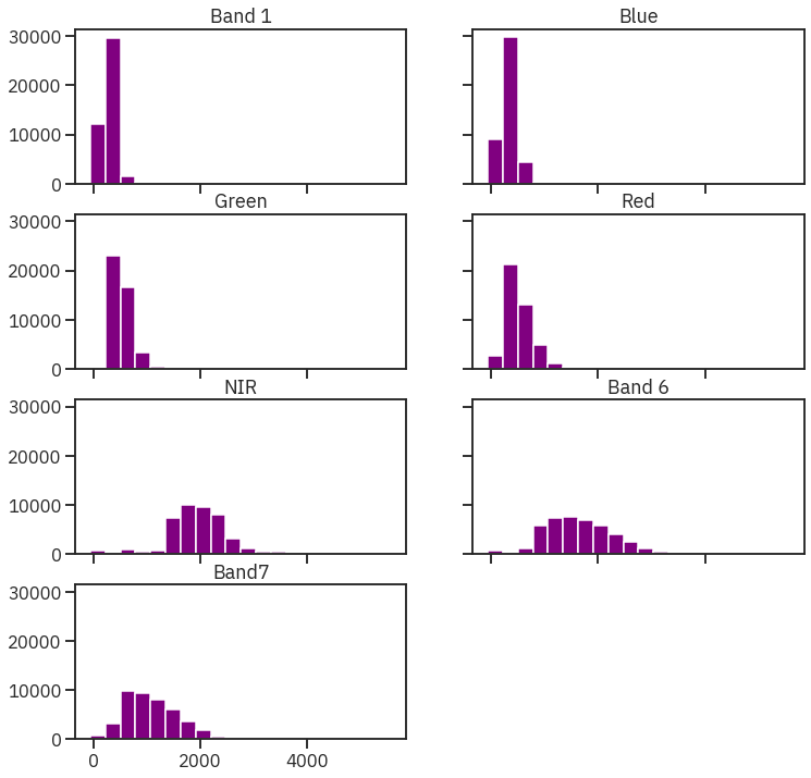
In [25]:
# Plot all band histograms using earthpy
band_titles = ["Band 1", "Blue", "Green", "Red",
               "NIR", "Band 6", "Band7"]

ep.hist(landsat_post_fire,
        title=band_titles)
Out[25]:
Crop single image
In [26]:
fire_boundary_path = os.path.join("data",
"cold-springs-fire",
"vector_layers",
"fire-boundary-geomac",
"co_cold_springs_20160711_2200_dd83.shp")
fire_boundary = gpd.read_file(fire_boundary_path)
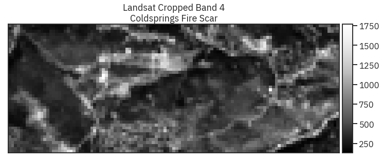
# Open a single band and plot
with rio.open(all_landsat_post_bands[3]) as src:
# Reproject the fire boundary shapefile to be the same CRS as the Landsat data
crop_raster_profile = src.profile
fire_boundary_utmz13 = fire_boundary.to_crs(crop_raster_profile["crs"])
# Crop the landsat image to the extent of the fire boundary
landsat_band4, landsat_metadata = es.crop_image(src, fire_boundary_utmz13)
ep.plot_bands(landsat_band4[0],
title="Landsat Cropped Band 4\nColdsprings Fire Scar",
scale=False)
Out[26]:
Crop all bands
In [27]:
cropped_folder = os.path.join("data",
                              "cold-springs-fire",
                              "outputs",
                              "cropped-images")

if not os.path.isdir(cropped_folder):
    os.mkdir(cropped_folder)

cropped_file_list = es.crop_all(all_landsat_post_bands,
                                cropped_folder,
                                fire_boundary_utmz13,
                                overwrite=True,
                                verbose=True)

cropped_file_list
Out[27]:
In [28]:
landsat_post_fire_path = os.path.join("data", "cold-springs-fire",
                                      "outputs", "landsat_post_fire.tif")

# This will create a new stacked raster with all bands
land_stack, land_meta = es.stack(cropped_file_list,
                                 landsat_post_fire_path)
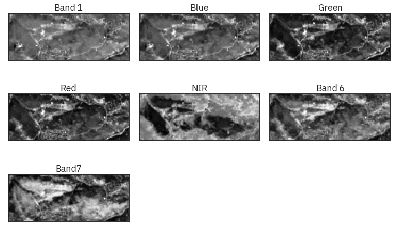
In [29]:
# Plot all bands using earthpy
band_titles = ["Band 1", "Blue", "Green", "Red",
               "NIR", "Band 6", "Band7"]

ep.plot_bands(land_stack,
              figsize=(11, 7),
              title=band_titles,
              cbar=False)
Out[29]:
Download from earthexplorer instructions: https://www.earthdatascience.org/courses/use-data-open-source-python/multispectral-remote-sensing/landsat-in-Python/get-landsat-data-earth-explorer/
NAIP
National Agriculture Imagery Program https://www.earthdatascience.org/courses/use-data-open-source-python/multispectral-remote-sensing/intro-naip/
In [40]:
from shapely.geometry import Polygon, mapping, box
import rasterio as rio
from rasterio.mask import mask
from rasterio.plot import show
from pprint import pprint
In [35]:
naip_csf_path = os.path.join("data", "cold-springs-fire",
                             "naip", "m_3910505_nw_13_1_20150919",
                             "crop", "m_3910505_nw_13_1_20150919_crop.tif")

with rio.open(naip_csf_path) as src:
    naip_csf = src.read()
    naip_csf_meta = src.meta
pprint(naip_csf_meta)
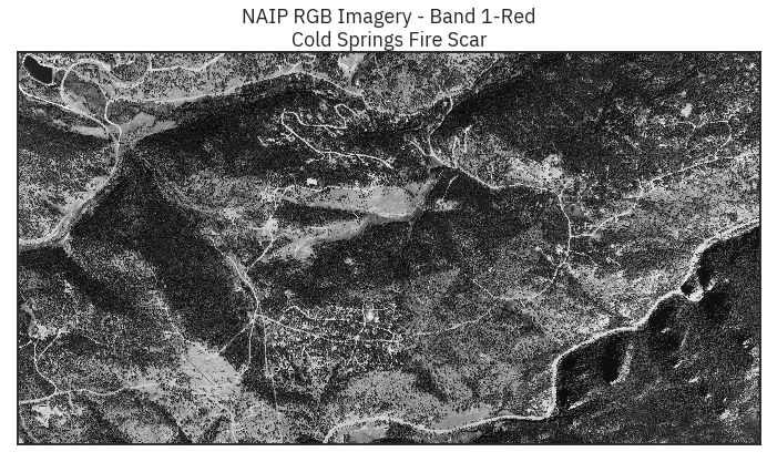
In [41]:
ep.plot_bands(naip_csf[0],
              title="NAIP RGB Imagery - Band 1-Red\nCold Springs Fire Scar",
              cbar=False)
Out[41]:
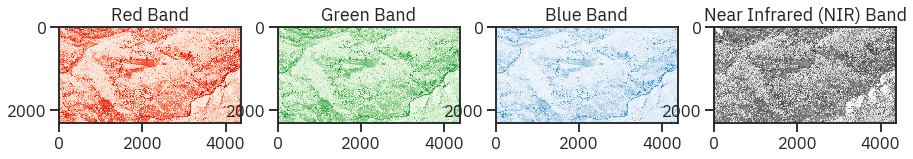
In [70]:
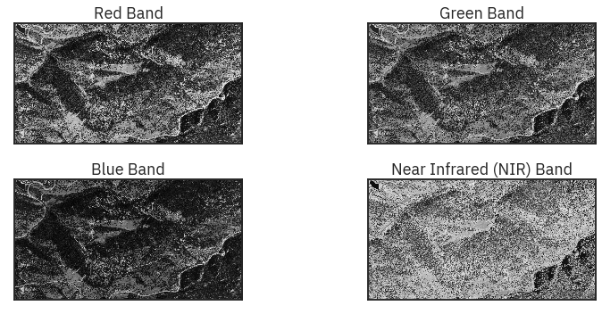
titles = ["Red Band", "Green Band", "Blue Band", "Near Infrared (NIR) Band"]
cmaps = ['Reds', 'Greens', 'Blues', 'Greys']
# f, ax = plt.subplots(2, 2, dpi = 140)
f, ax = plt.subplots(1, 4, figsize = (15, 5))
for ax, i in zip(ax, np.arange(0, 4)):
    ax.imshow(naip_csf[i], cmap = cmaps[i])
    ax.set_title(titles[i])
Out[70]:
Out[70]:
Out[70]:
Out[70]:
Out[70]:
Out[70]:
Out[70]:
Out[70]:
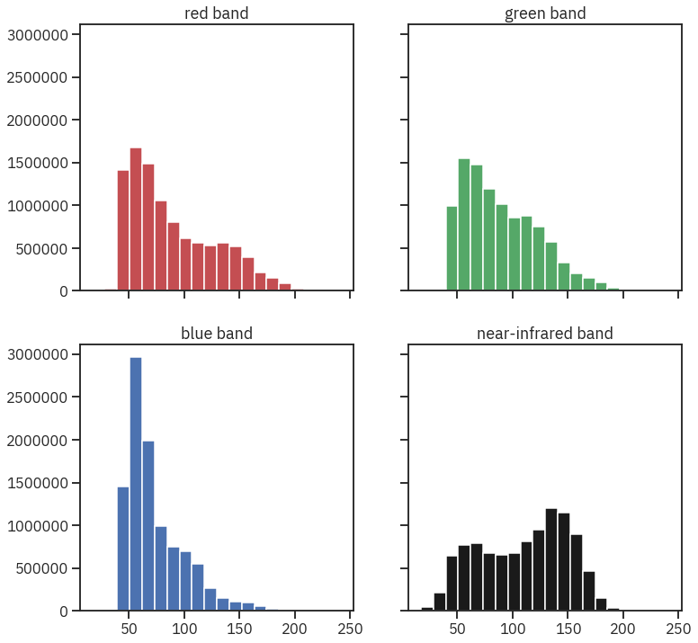
In [72]:
colors = ['r', 'g', 'b', 'k']
titles = ['red band', 'green band', 'blue band', 'near-infrared band']

ep.hist(naip_csf,
        colors=colors,
        title=titles,
        cols=2)

plt.show()
Out[72]:
In [71]:
ep.plot_bands(naip_csf,
figsize=(12, 5),
cols=2,
title=titles,
cbar=False)
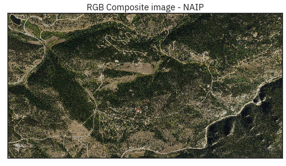
ep.plot_rgb(naip_csf,
rgb=[0, 1, 2],
title="RGB Composite image - NAIP")
Out[71]:
Out[71]: