In [1]:
import os, sys, glob
from pathlib import Path
import numpy as np
import pandas as pd
import seaborn as sns

import matplotlib.pyplot as plt
from IPython.core.interactiveshell import InteractiveShell
InteractiveShell.ast_node_interactivity = 'all'
In [2]:
from sympy import *
var('x, y, z, a, b, c, α, β, γ, σ')
init_printing()
Out[2]:
In [3]:
1 + 1
1 * 2
3 ** 2
3 / 2
3 // 2 # integer division
9 % 5  # modulo
Out[3]:
Out[3]:
Out[3]:
Out[3]:
Out[3]:
Out[3]:
Data types
In [4]:
type(3)
type(3.5)
int(3.8)
Out[4]:
Out[4]:
Out[4]:
Native fractions
In [5]:
from fractions import Fraction
In [6]:
f = Fraction(2, 3)
f + 1
Out[6]:
Complex numbers
In [7]:
a = 2 + 3j
a
Out[7]:
User input
In [8]:
a = float(input())
In [9]:
a + 1
Out[9]:
Exception Handling
In [10]:
 try:
    a = float(input('Enter a number: '))
except ValueError:
    print('You entered an invalid number')
Functions
In [11]:
def multi_table(a):
     for i in range(1, 11):
        print(f'{a} x {i} = {a*i}')
In [12]:
multi_table(5)
solve for x $a x^2 + b x + c = 0$
$$ x = \frac{- b \pm \sqrt{b^2 - 4ac}}{2a} $$In [13]:
def quad_solver(a, b, c):
    D = (b**2 - 4*a*c)**.5
    return([ (-b + D) / (2*a), (-b - D) / (2*a) ])
In [14]:
quad_solver(4,5,-2)
Out[14]:
In [15]:
from pylab import plot, show
In [16]:
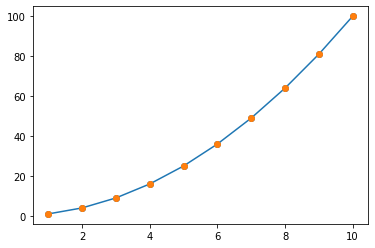
x = range(1, 11)
y = [x**2 for x in x]
plot(x, y, marker = 'o')

plot(x, y, 'o')
Out[16]:
Out[16]:
In [17]:
# 2. Define data
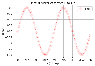
x = np.arange(0, 4 * np.pi, 0.2)
y = np.sin(x)
# 3. Plot data including options
plt.plot(x, y,
linewidth=0.5,
linestyle='--',
color='r',
marker='o',
markersize=10,
markerfacecolor=(1, 0, 0, 0.1))
# 4. Add plot details
plt.title('Plot of sin(x) vs x from 0 to 4 pi')
plt.xlabel('x (0 to 4 pi)')
plt.ylabel('sin(x)')
plt.legend(['sin(x)']) # list containing one string
plt.xticks(
np.arange(0, 4*np.pi + np.pi/2, np.pi/2),
['0','pi/2','pi','3pi/2','2pi','5pi/2','3pi','7pi/2','4pi'])
plt.grid(True)
# 5. Show the plot
plt.show()
Out[17]:
Out[17]:
Out[17]:
Out[17]:
Out[17]:
Out[17]:
save figure
plt.savefig('plot.png', dpi=300, bbox_inches='tight')
Multiple Series
In [18]:
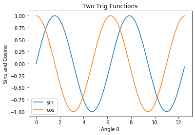
x = np.arange(0,4*np.pi,0.1)
y = np.sin(x)
z = np.cos(x)


f, ax = plt.subplots()


ax.plot(x,y)
ax.plot(x,z)


ax.set_title('Two Trig Functions')
ax.legend(['sin','cos'])
ax.xaxis.set_label_text('Angle θ')
ax.yaxis.set_label_text('Sine and Cosine')
Out[18]:
Out[18]:
Out[18]:
Out[18]:
Out[18]:
Out[18]:
Other Plots
Scatterplot
In [19]:
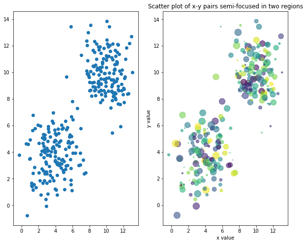
# random but semi-focused data
x1 = 1.5 * np.random.randn(150) + 10
y1 = 1.5 * np.random.randn(150) + 10
x2 = 1.5 * np.random.randn(150) + 4
y2 = 1.5 * np.random.randn(150) + 4
x = np.append(x1,x2)
y = np.append(y1,y2)
In [20]:
colors = np.random.rand(150*2)
area = np.pi * (8 * np.random.rand(150*2))**2
In [21]:
fig, ax = plt.subplots(1, 2, figsize = (10, 8))
ax[0].scatter(x,y)

ax[1].scatter(x, y, s=area, c=colors, alpha=0.6)
ax[1].set_title('Scatter plot of x-y pairs semi-focused in two regions')
ax[1].set_xlabel('x value')
ax[1].set_ylabel('y value')
Out[21]:
Out[21]:
Out[21]:
Out[21]:
Out[21]:
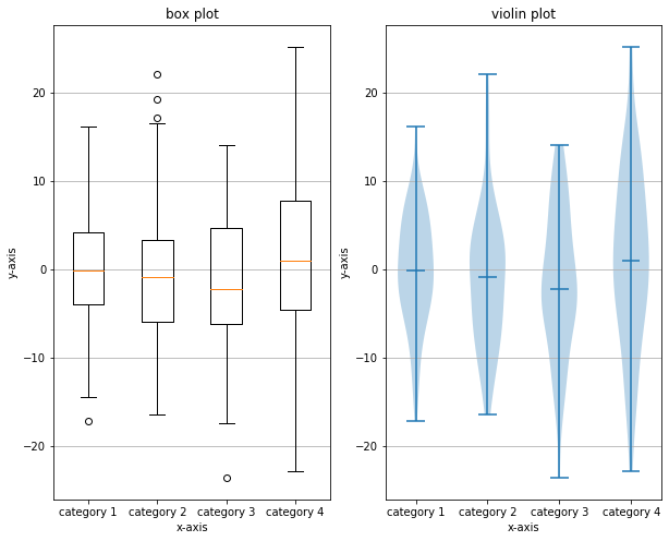
Boxplots / Violin Plots
In [22]:
# generate some random data
data1 = np.random.normal(0, 6, 100)
data2 = np.random.normal(0, 7, 100)
data3 = np.random.normal(0, 8, 100)
data4 = np.random.normal(0, 9, 100)
data = list([data1, data2, data3, data4])
In [23]:
fig, ax = plt.subplots(1, 2, figsize = (10, 8))


# build a box plot
ax[0].boxplot(data)


# title and axis labels
ax[0].set_title('box plot')
ax[0].set_xlabel('x-axis')
ax[0].set_ylabel('y-axis')
xticklabels=['category 1', 'category 2', 'category 3', 'category 4']
ax[0].set_xticklabels(xticklabels)


# add horizontal grid lines
ax[0].yaxis.grid(True)

# build a violin plot
ax[1].violinplot(data, showmeans=False, showmedians=True)

# add title and axis labels
ax[1].set_title('violin plot')
ax[1].set_xlabel('x-axis')
ax[1].set_ylabel('y-axis')


# add x-tick labels
xticklabels = ['category 1', 'category 2', 'category 3', 'category 4']
ax[1].set_xticks([1,2,3,4])
ax[1].set_xticklabels(xticklabels)


# add horizontal grid lines
ax[1].yaxis.grid(True)
Out[23]:
Out[23]:
Out[23]:
Out[23]:
Out[23]:
Out[23]:
Out[23]:
Out[23]:
Out[23]:
Out[23]:
Out[23]:
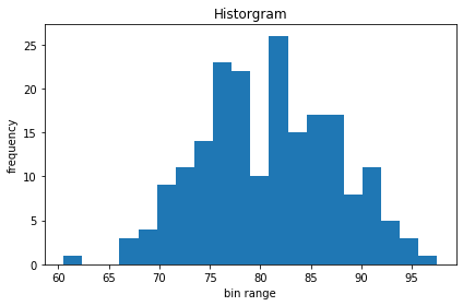
Histogram
In [24]:
mu = 80
sigma = 7
x = np.random.normal(mu, sigma, size=200)


fig, ax = plt.subplots()


ax.hist(x, 20)
ax.set_title('Historgram')
ax.set_xlabel('bin range')
ax.set_ylabel('frequency')


fig.tight_layout()
Out[24]:
Out[24]:
Out[24]:
Out[24]:
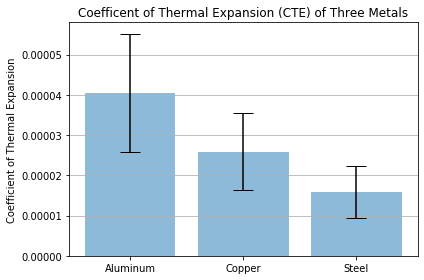
Bar Plot
In [25]:
# Data
aluminum = np.array([
    6.4e-5, 3.01e-5, 2.36e-5, 3.0e-5, 7.0e-5, 4.5e-5, 3.8e-5, 4.2e-5, 2.62e-5,
    3.6e-5
])
copper = np.array([
    4.5e-5, 1.97e-5, 1.6e-5, 1.97e-5, 4.0e-5, 2.4e-5, 1.9e-5, 2.41e-5, 1.85e-5,
    3.3e-5
])
steel = np.array([
    3.3e-5, 1.2e-5, 0.9e-5, 1.2e-5, 1.3e-5, 1.6e-5, 1.4e-5, 1.58e-5, 1.32e-5,
    2.1e-5
])
# Create arrays for the plot
materials = ['Aluminum', 'Copper', 'Steel']
x_pos = np.arange(len(materials))
aluminum_mean = np.mean(aluminum)
copper_mean = np.mean(copper)
steel_mean = np.mean(steel)
# Calculate the standard deviation
aluminum_std = np.std(aluminum)
copper_std = np.std(copper)
steel_std = np.std(steel)

CTEs = [aluminum_mean, copper_mean, steel_mean]
error = [aluminum_std, copper_std, steel_std]


# Build the plot
fig, ax = plt.subplots()

ax.bar(x_pos, CTEs,
       yerr=error,
       align='center',
       alpha=0.5,
       ecolor='black',
       capsize=10)
ax.set_ylabel('Coefficient of Thermal Expansion')
ax.set_xticks(x_pos)
ax.set_xticklabels(materials)
ax.set_title('Coefficent of Thermal Expansion (CTE) of Three Metals')
ax.yaxis.grid(True)


# Save the figure and show
plt.tight_layout()
Out[25]:
Out[25]:
Out[25]:
Out[25]:
Out[25]:
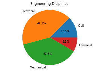
Pie Chart (never use)
In [26]:
# Pie chart, where the slices will be ordered and plotted counter-clockwise:
labels = ['Civil', 'Electrical', 'Mechanical', 'Chemical']
sizes = [15, 50, 45, 10]


fig, ax = plt.subplots()
ax.pie(sizes, labels=labels, autopct='%1.1f%%')
ax.axis('equal')  # Equal aspect ratio ensures the pie chart is circular.
ax.set_title('Engineering Diciplines')
Out[26]:
Out[26]:
Out[26]:
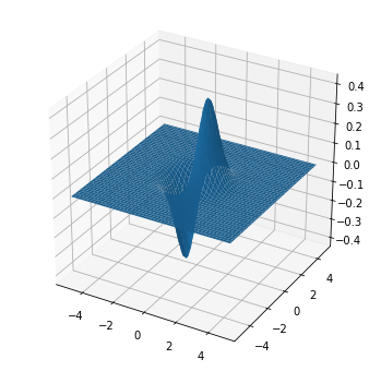
Surface Plot
In [27]:
from mpl_toolkits.mplot3d import axes3d
x = np.arange(-5,5,0.1)
y = np.arange(-5,5,0.1)
X,Y = np.meshgrid(x,y)
Z = X*np.exp(-X**2 - Y**2)

fig = plt.figure(figsize=(6,6))
ax = fig.add_subplot(111, projection='3d')

# Plot a 3D surface
ax.plot_surface(X, Y, Z)
Out[27]:
Basic Statistics
In [28]:
man_mean = lambda x: sum(x)/len(x)
In [29]:
def man_median(num):
    num.sort()
    l = len(num)
    if l % 2 == 0:
        med = num[int(l/2)]
    else:
        med = num[int(l/2 + 1)]
    return med
In [30]:
sc = [100, 60, 70, 900, 100, 200, 500, 500, 503, 600, 1000, 1200]
man_mean(sc)
np.mean(sc)
man_median(sc)
np.median(sc)
Out[30]:
Out[30]:
Out[30]:
Out[30]:
In [31]:
from collections import Counter
def man_mode(num):
    c = Counter(num)
    return c.most_common(1)[0][0]
In [32]:
scores = [7, 8, 9, 2, 10, 9, 9, 9, 9, 4, 5, 6, 1, 5, 6, 7, 8, 6, 1, 10]
man_mode(scores)
Out[32]:
In [33]:
def freq_table(num):
    c = Counter(num)
    ftable = '\n'.join([f'{n[0]}\t{n[1]}' for n in c.most_common()])
    return ftable
In [34]:
print(freq_table(scores))
In [35]:
man_range = lambda num: max(num) - min(num)
man_range(scores)
Out[35]:
Sympy
In [36]:
from sympy import *
init_printing()
var('x, y, z, α, β, γ, φ, ω, ε')
a, b, c, k, m, n = symbols('a b c k m n', integer=True)
f, g, h = symbols('f g h', cls=Function)
Out[36]:
Elementary
Expressions
In [37]:
Rational(3, 2)*pi + exp(I * x) / (x**2 + y)
Out[37]:
Evaluate at value
In [38]:
exp(I*x).subs(x,pi).evalf()
Out[38]:
In [39]:
expr = (x + y) ** 2
expr.expand()
Out[39]:
Factor or Substitute Expressions
In [40]:
exp = x**2 + 5*x + 3
exp
Out[40]:
In [41]:
e = x**2 - y**2
e.factor()
e.subs({x : 4, y : 1 - x})
Out[41]:
Out[41]:
In [42]:
limit(1/x,x,0,dir="-")
Out[42]:
In [43]:
limit(1/x**2,x,0,dir='+')
Out[43]:
Solvers
Single variable equation
In [44]:
exp = x**2 + 5*x + 3
exp
Out[44]:
In [45]:
solve(exp, x)
Out[45]:
In [46]:
exp = Eq(x**2 + 5*x + 3, 0)
exp
solve(exp)
Out[46]:
Out[46]:
In [47]:
solve(a * x **2 + b * x + c, x)
solveset(a * x **2 + b * x + c, x)
Out[47]:
Out[47]:
Solve with specific domain
In [48]:
solveset(x ** 2 + 1, x, domain=S.Reals)
Out[48]:
System of Equations
In [49]:
solve([x + 5*y - 2, -3*x + 6*y - 15], [x, y], dict = True)
Out[49]:
In [50]:
eq1 = Eq(x + y - 5, 0)
eq2 = Eq(x - y + 3, 0)
solve((eq1, eq2), (x, y))
Out[50]:
Single Inequality
In [51]:
ineq = (10000 / x) - 1 < 0
solveset(ineq, x, S.Reals)
Out[51]:
System of inequalities
In [52]:
from sympy.solvers.inequalities import *
In [53]:
reduce_inequalities([x + 4*y - 2 > 0,
                     x - 3 + 2*y <= 5],
                    [x])
Out[53]:
In [54]:
from sympy.polys import Poly
solve_poly_inequalities(((
    Poly(x**2 - 3), "<"), (
    Poly(-x**2 + 1), ">")))
Out[54]:
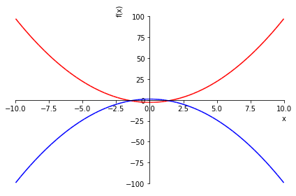
Verify graphically
In [55]:
p = plot(x**2 - 3, -x**2 + 1, show = False)
p[0].line_color = 'r'
p[1].line_color = 'b'
p.show()
Sums and Products
In [56]:
a, b = symbols('a b')
s = Sum(6*n**2 + 2**n, (n, a, b))
s
s.doit()
Out[56]:
Out[56]:
In [57]:
p = product(n*(n+1), (n, 1, b))
p
p.doit()
Out[57]:
Out[57]:
Calculus
In [58]:
limit((sin(x)-x)/x**3, x, 0)
Out[58]:
In [59]:
diff(cos(x**2)**2 / (1+x), x)
Out[59]:
In [60]:
integrate(x**2 * cos(x), x)
Out[60]:
In [61]:
integrate(x**2 * cos(x), (x, 0, pi/2))
Out[61]:
Differential Equations
In [62]:
dsolve(Eq(Derivative(f(x),x,x) + 9*f(x), 1), f(x))
Out[62]:
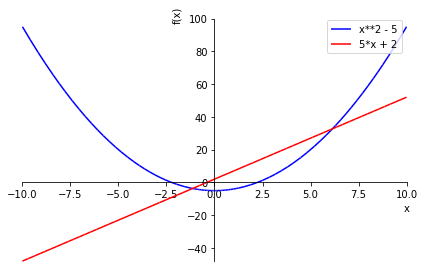
Plot multiple functions with labels
In [63]:
from sympy.plotting import plot
In [64]:
p = plot(x ** 2 - 5, 5*x + 2, legend = True, show = False)
p[0].line_color = 'b'
p[1].line_color = 'r'
p.show()
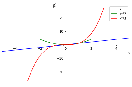
In [65]:
p = plot( (x, (x,-5,5)), (x**2, (x,-2,2)), (x**3, (x,-3,3)),
    xlabel='x',
    ylabel='f(x)', legend = True, show = False)
p[0].line_color = 'b'
p[1].line_color = 'g'
p[2].line_color = 'r'
p.show()
Sets and Probability
In [66]:
s = FiniteSet(2, 4, 6)
s
Out[66]:
In [67]:
{'apple', 'orange', 'apple', 'pear', 'orange', 'banana'}
Out[67]:
In [68]:
4 in s
Out[68]:
Numpy
In [69]:
np.array([1,2,3])
Out[69]:
Basic Arrays
regularly spaced
arange(start, stop, step)
In [70]:
np.arange(0, 10+2, 2)
Out[70]:
np.linspace(start, stop, number of elements)
In [71]:
np.linspace(0,2*np.pi,10)
Out[71]:
np.logspace(start, stop, number of elements, base=<num>)
In [72]:
np.logspace(1, 2, 5 )
Out[72]:
Matrices
my_array = np.zeros((rows,cols))
In [73]:
np.zeros((5,5))
Out[73]:
my_array = np.ones((rows,cols))
In [74]:
np.ones((3,5))
Out[74]:
np.eye(dim)
In [75]:
np.eye(5)
Out[75]:
Meshgrid / np.mgrid[]
In [76]:
X, Y = np.mgrid[0:5,0:11:2]
print(X)
print(Y)
Random Numbers Generation
Random Integers
np.random.randint(lower limit, upper limit, number of values)
In [77]:
np.random.randint(0,10,5)
Out[77]:
Random numbers on unit interval np.random.rand(number of values)
In [78]:
np.random.rand(5)
Out[78]:
Random choice np.random.choice(list of choices, number of choices)
In [79]:
lst = [1,5,9,11]
np.random.choice(lst,3)
Out[79]:
Draw from Standard Normal distribution np.random.randn(number of values)
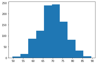
In [80]:
np.random.randn(10)
μ = 70
σ = 6.6

sample = [σ * np.random.randn(1000) + μ]
Out[80]:
In [81]:
plt.hist(sample)
Out[81]:
Indexing / Slicing
In [82]:
a = np.array([[2,3,4],[6,7,8]])
a
a[1,2]
Out[82]:
Out[82]:
In [83]:
a = np.array([2, 4, 6])
a
a[:2]
Out[83]:
Out[83]:
In [84]:
a = np.array([[2, 4, 6, 8], [10, 20, 30, 40]])
a
a[0:2, 0:3]
a[:2, :]  #[first two rows, all columns]
Out[84]:
Out[84]:
Out[84]:
Vector operations
Scalar operations
In [85]:
a = np.array([1, 2, 3])
a + 2
a * 3
Out[85]:
Out[85]:
Vec operations
In [86]:
a = np.array([1, 2, 3])
b = np.array([4, 5, 6])
a * b
np.dot(a, b)
np.cross(a, b)
Out[86]:
Out[86]:
Out[86]:
In [87]:
a = np.array([1, 2, 3])
np.exp(a)
np.log(a)
np.log(np.e)
np.log10(1000)
Out[87]:
Out[87]:
Out[87]:
Out[87]:
Trig
In [88]:
a = np.array([0, np.pi/4, np.pi/3, np.pi/2])
print(np.sin(a))
print(np.cos(a))
print(np.tan(a))
System of Equations
In [89]:
A = np.array([[8, 3, -2], [-4, 7, 5], [3, 4, -12]])
A
b = np.array([9, 15, 35])
b
np.linalg.solve(A, b)
Out[89]:
Out[89]:
Out[89]:
In [ ]: