Introduction to Spatial Data Analysis in Python
import os, sys, glob
from pathlib import Path
import numpy as np
import pandas as pd
import seaborn as sns

import matplotlib.pyplot as plt

# vector / visualisation packages
import geopandas as gpd
import geoplot as gplt
import mapclassify as mc
import geoplot.crs as gcrs
from earthpy import clip as cl

# raster packages
import rasterio as rio
import georasters as gr
from rasterstats import zonal_stats

# spatial econometrics
import pysal as ps
import esda
import libpysal as lps
from pysal.lib.weights.weights import W


from IPython.core.interactiveshell import InteractiveShell
InteractiveShell.ast_node_interactivity = 'all'
Vector data
From Natural Earth
cities = gpd.read_file("https://www.naturalearthdata.com/http//www.naturalearthdata.com/download/110m/cultural/ne_110m_populated_places.zip")
countries = gpd.read_file('https://www.naturalearthdata.com/http//www.naturalearthdata.com/download/10m/cultural/ne_10m_admin_0_countries.zip')
countries.head()
cities.head()
Constructing Geodataframe from lon-lat
df = pd.DataFrame({'City': ['Buenos Aires', 'Brasilia', 'Santiago', 'Bogota', 'Caracas'],
     'Country': ['Argentina', 'Brazil', 'Chile', 'Colombia', 'Venezuela'],
     'Latitude': [-34.58, -15.78, -33.45, 4.60, 10.48],
     'Longitude': [-58.66, -47.91, -70.66, -74.08, -66.86]})
lat_am_capitals = gpd.GeoDataFrame(df, geometry = gpd.points_from_xy(df.Longitude, df.Latitude))
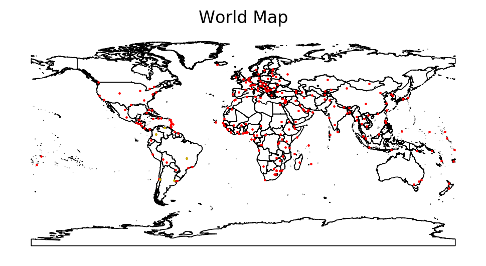
Making Maps
f, ax = plt.subplots(dpi = 200)
countries.plot(edgecolor = 'k', facecolor = 'None', linewidth = 0.6, ax = ax)
cities.plot(markersize = 0.5, facecolor = 'red', ax = ax)
lat_am_capitals.plot(markersize = 0.5, facecolor = 'y', ax = ax)
ax.set_title('World Map')
ax.set_axis_off()
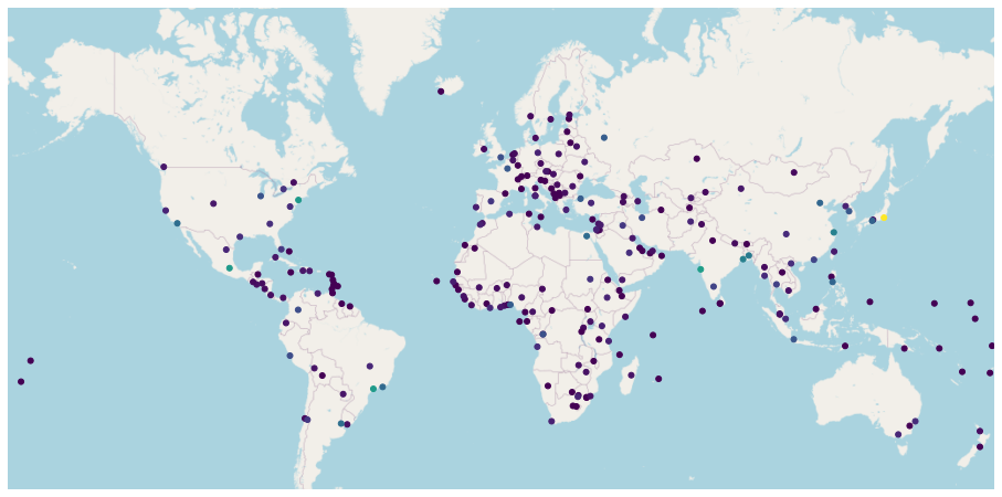
Static Webmaps
ax = gplt.webmap(countries, projection=gplt.crs.WebMercator(), figsize = (16, 12))
gplt.pointplot(cities, ax=ax, hue = 'POP2015')
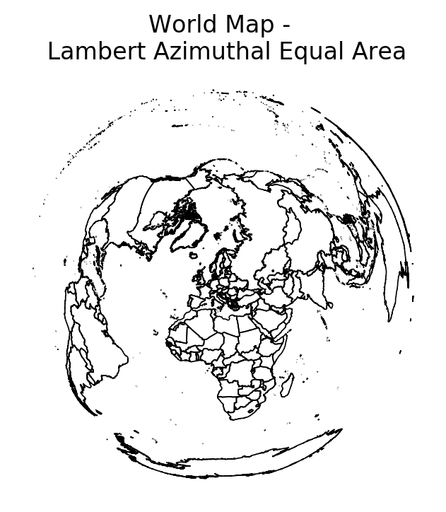
Aside on Projections
Map projections flatten a globe's surface onto a 2D plane. This necessarily distorts the surface (one of Gauss' lesser known results), so one must choose specific form of 'acceptable' distortion.
By convention, the standard projection in GIS is World Geodesic System(lat/lon - WGS84). This is a cylindrical projection, which stretches distances east-west and results in incorrect distance and areal calculations. For accurate distance and area calculations, try to use UTM (which divides map into zones). See epsg.io
countries.crs
countries_2 = countries.copy()
countries_2 = countries_2.to_crs({'init': 'epsg:3035'})
f, ax = plt.subplots(dpi = 200)
countries_2.plot(edgecolor = 'k', facecolor = 'None', linewidth = 0.6, ax = ax)
ax.set_title('World Map - \n Lambert Azimuthal Equal Area')
ax.set_axis_off()
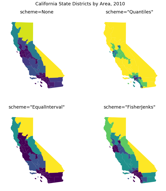
Choropleths
Maps with color-coding based on value in table
- scheme=None—A continuous colormap.
- scheme=”Quantiles”—Bins the data such that the bins contain equal numbers of samples.
- scheme=”EqualInterval”—Bins the data such that bins are of equal length.
- scheme=”FisherJenks”—Bins the data using the Fisher natural breaks optimization procedure.
(Example from geoplots gallery)
cali = gpd.read_file(gplt.datasets.get_path('california_congressional_districts'))
cali['area'] =cali.geometry.area

proj=gcrs.AlbersEqualArea(central_latitude=37.16611, central_longitude=-119.44944)
fig, axarr = plt.subplots(2, 2, figsize=(12, 12), subplot_kw={'projection': proj})

gplt.choropleth(
    cali, hue='area', linewidth=0, scheme=None, ax=axarr[0][0]
)
axarr[0][0].set_title('scheme=None', fontsize=18)

scheme = mc.Quantiles(cali.area, k=5)
gplt.choropleth(
    cali, hue='area', linewidth=0, scheme=scheme, ax=axarr[0][1]
)
axarr[0][1].set_title('scheme="Quantiles"', fontsize=18)

scheme = mc.EqualInterval(cali.area, k=5)
gplt.choropleth(
    cali, hue='area', linewidth=0, scheme=scheme, ax=axarr[1][0]
)
axarr[1][0].set_title('scheme="EqualInterval"', fontsize=18)

scheme = mc.FisherJenks(cali.area, k=5)
gplt.choropleth(
    cali, hue='area', linewidth=0, scheme=scheme, ax=axarr[1][1]
)
axarr[1][1].set_title('scheme="FisherJenks"', fontsize=18)

plt.subplots_adjust(top=0.92)
plt.suptitle('California State Districts by Area, 2010', fontsize=18)
Spatial Merge
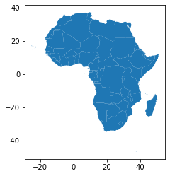
Subset to Africa
afr = countries.loc[countries.CONTINENT == 'Africa']
afr.plot()
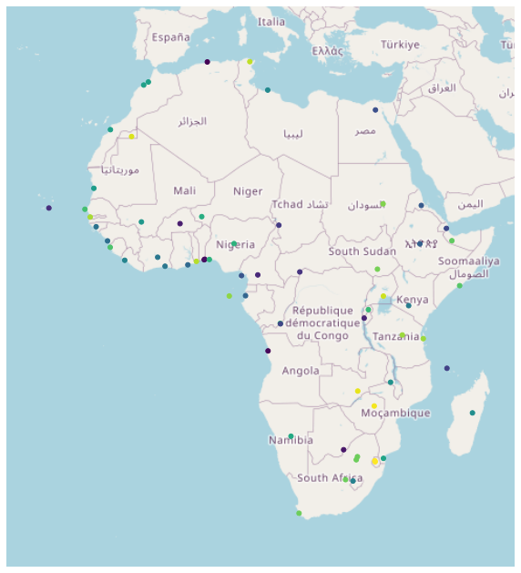
Subset cities by merging with African boundaries
afr_cities = gpd.sjoin(cities, afr, how='inner')
ax = gplt.webmap(afr, projection=gplt.crs.WebMercator(), figsize = (10, 14))
gplt.pointplot(afr_cities, ax=ax, hue = 'NAME_EN')
afr_cities.head()
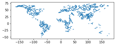
Distance Calculations
rivers = gpd.read_file('https://www.naturalearthdata.com/http//www.naturalearthdata.com/download/50m/physical/ne_50m_rivers_lake_centerlines.zip')
rivers.geometry.head()
rivers.plot()
def min_distance(point, lines = rivers):
    return lines.distance(point).min()

afr_cities['min_dist_to_rivers'] = afr_cities.geometry.apply(min_distance)
f, ax = plt.subplots(dpi = 200)
afr.plot(edgecolor = 'k', facecolor = 'None', linewidth = 0.6, ax = ax)
rivers.plot(ax = ax, linewidth = 0.5)
afr_cities.plot(column = 'min_dist_to_rivers', markersize = 0.9, ax = ax)
ax.set_ylim(-35, 50)
ax.set_xlim(-20, 55)
ax.set_title('Cities by shortest distance to Rivers')
ax.set_axis_off()

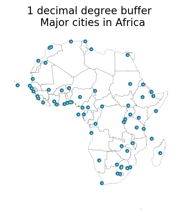
Buffers
afr_cities_buf = afr_cities.buffer(1)
f, ax = plt.subplots(dpi = 200)
afr.plot(facecolor = 'None', edgecolor = 'k', linewidth = 0.1, ax = ax)
afr_cities_buf.plot(ax=ax, linewidth=0)
afr_cities.plot(ax=ax, markersize=.2, color='yellow')
ax.set_title('1 decimal degree buffer \n Major cities in Africa', fontsize = 12)
ax.set_axis_off()
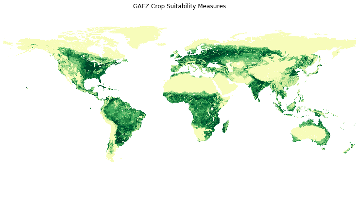
Raster Data
raster = 'data/res03_crav6190h_sihr_cer.tif'
# Get info on raster
NDV, xsize, ysize, GeoT, Projection, DataType = gr.get_geo_info(raster)

grow = gr.load_tiff(raster)
grow = gr.GeoRaster(grow, GeoT, projection = Projection)
f, ax = plt.subplots(1, figsize=(13, 11))
grow.plot(ax = ax, cmap = 'YlGn_r')
ax.set_title('GAEZ Crop Suitability Measures')
ax.set_axis_off()
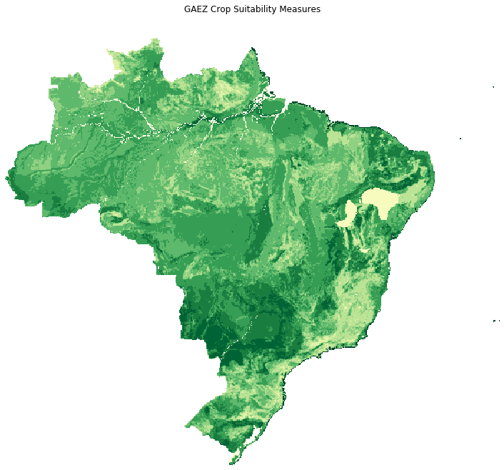
Clipping Raster
brazil = countries.query('ADMIN == "Brazil"')
grow_clip = grow.clip(brazil)[0]
f, ax = plt.subplots(1, figsize=(13, 11))
grow_clip.plot(ax = ax, cmap = 'YlGn_r')
ax.set_title('GAEZ Crop Suitability Measures')
ax.set_axis_off()
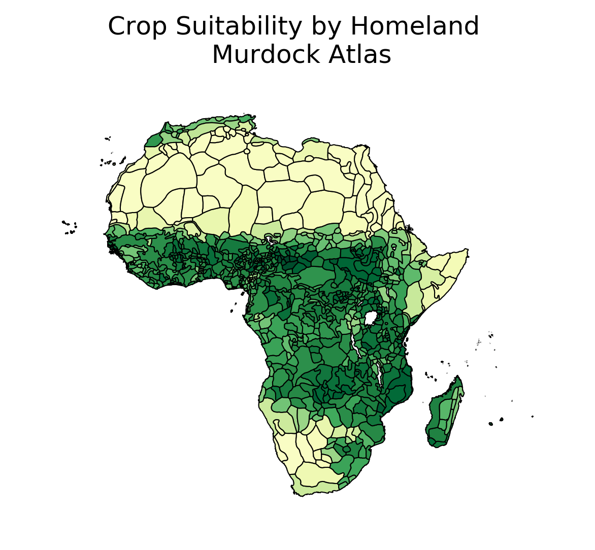
Zonal Statistics
murdock = gpd.read_file('https://scholar.harvard.edu/files/nunn/files/murdock_shapefile.zip')
murdock_cs = gpd.GeoDataFrame.from_features((zonal_stats(murdock, raster, geojson_out = True)))
f, ax = plt.subplots(dpi = 300)
gplt.choropleth(
    murdock_cs, hue='mean', linewidth=.5, cmap='YlGn_r', ax=ax
)
ax.set_title('Crop Suitability by Homeland \n Murdock Atlas', fontsize = 12)
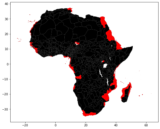
Spatial Econometrics
Weight Matrices
%time w = lps.weights.Queen.from_dataframe(murdock_cs)
w.n
w.mean_neighbors
ax = murdock_cs.plot(color='k', figsize=(9, 9))
murdock_cs.loc[w.islands, :].plot(color='red', ax=ax);
mur = murdock_cs.drop(w.islands)
%time w = lps.weights.Queen.from_dataframe(mur)
w.transform = 'r'
Moran's I
Measure of spatial correlation
$$I = \frac{N}{W} \frac{\sum_i \sum_j w_{ij} (x_i - \bar{x} ) ( x_j - \bar{x} ) }{ \sum_i (x_i - \bar{x})^2 }$$where $N$ is the total number of units, $x$ is the variable of interest, $w_{ij}$ is the spatial weight between units $i$ and $j$, and $W$ is the sum of all weights $w_{ij}$
$I \in [-1, 1]$. Under null of no spatial correlation, $E(I) = \frac{-1}{N-1} \rightarrow 0$ with large $N$.
mur.shape
mi = esda.moran.Moran(mur['mean'], w)
mi.I
mi.p_sim
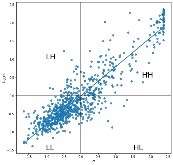
Spatial Lag
mur['cs'] = (mur['mean'] - mur['mean'].mean()) / mur['mean'].std()
mur['lag_cs'] = lps.weights.lag_spatial(w, mur['cs'])
f, ax = plt.subplots(1, figsize=(9, 9))
# Plot values
sns.regplot(x='cs', y='lag_cs', data=mur, ci=None)
# Add vertical and horizontal lines
plt.axvline(0, c='k', alpha=0.5)
plt.axhline(0, c='k', alpha=0.5)
plt.text(1.75, 0.5, "HH", fontsize=25)
plt.text(1.5, -1.5, "HL", fontsize=25)
plt.text(-1, 1, "LH", fontsize=25)
plt.text(-1.0, -1.5, "LL", fontsize=25)
# Display
plt.show()
More
- Local Indicators of Spatial Autocorrelation (spatial clustering)
- Conley SEs
- Gaussian Random Fields