Databases in R

In [43]:
rm(list = ls())
library(LalRUtils)
libreq(data.table, magrittr, tidyverse, janitor, huxtable, knitr, tictoc)
theme_set(lal_plot_theme_d())
options(repr.plot.width = 15, repr.plot.height=12)
     wants        loaded
[1,] "data.table" TRUE  
[2,] "magrittr"   TRUE  
[3,] "tidyverse"  TRUE  
[4,] "janitor"    TRUE  
[5,] "huxtable"   TRUE  
[6,] "knitr"      TRUE  
[7,] "tictoc"     TRUE  

Basics

In [44]:
libreq(tidyverse, DBI, dbplyr, RSQLite, bigrquery, hrbrthemes, nycflights13, glue)
     wants          loaded
[1,] "tidyverse"    TRUE  
[2,] "DBI"          TRUE  
[3,] "dbplyr"       TRUE  
[4,] "RSQLite"      TRUE  
[5,] "bigrquery"    TRUE  
[6,] "hrbrthemes"   TRUE  
[7,] "nycflights13" TRUE  
[8,] "glue"         TRUE  
In [45]:
con <- dbConnect(RSQLite::SQLite(), path = ":memory:")
In [46]:
copy_to(
  dest = con, 
  df = nycflights13::flights, 
  name = "flights",
  temporary = FALSE, 
  indexes = list(
    c("year", "month", "day"), 
    "carrier", 
    "tailnum",
    "dest"
    )
  )
In [47]:
flights_db <- tbl(con, "flights")
flights_db %>% head
# Source:   lazy query [?? x 19]
# Database: sqlite 3.30.1 []
   year month   day dep_time sched_dep_time dep_delay arr_time sched_arr_time
  <int> <int> <int>    <int>          <int>     <dbl>    <int>          <int>
1  2013     1     1      517            515         2      830            819
2  2013     1     1      533            529         4      850            830
3  2013     1     1      542            540         2      923            850
4  2013     1     1      544            545        -1     1004           1022
5  2013     1     1      554            600        -6      812            837
6  2013     1     1      554            558        -4      740            728
# … with 11 more variables: arr_delay <dbl>, carrier <chr>, flight <int>,
#   tailnum <chr>, origin <chr>, dest <chr>, air_time <dbl>, distance <dbl>,
#   hour <dbl>, minute <dbl>, time_hour <dbl>

dplyr code that is SQL in disguise

In [48]:
tailnum_delay_db <- 
  flights_db %>% 
  group_by(tailnum) %>%
  summarise(
    mean_dep_delay = mean(dep_delay),
    mean_arr_delay = mean(arr_delay),
    n = n()
    ) %>% 
  arrange(desc(mean_arr_delay)) %>%
  filter(n > 100)
tailnum_delay_db %>% show_query()
<SQL>
Warning message:
“Missing values are always removed in SQL.
Use `mean(x, na.rm = TRUE)` to silence this warning
This warning is displayed only once per session.”
SELECT *
FROM (SELECT *
FROM (SELECT `tailnum`, AVG(`dep_delay`) AS `mean_dep_delay`, AVG(`arr_delay`) AS `mean_arr_delay`, COUNT() AS `n`
FROM `flights`
GROUP BY `tailnum`)
ORDER BY `mean_arr_delay` DESC)
WHERE (`n` > 100.0)

Run SQL code directly

Using glue to stitch together a query

In [50]:
## Some local R variables
tbl <- "flights"
d_var <- "dep_delay"
d_thresh <- 240

## The "glued" SQL query string
sql_query <-
  glue_sql("
  SELECT *
  FROM {`tbl`}
  WHERE ({`d_var`} > {d_thresh})
  LIMIT 5
  ", 
  .con = con
  )

## Run the query
dbGetQuery(con, sql_query)
A data.frame: 5 × 19
yearmonthdaydep_timesched_dep_timedep_delayarr_timesched_arr_timearr_delaycarrierflighttailnumorigindestair_timedistancehourminutetime_hour
<int><int><int><int><int><dbl><int><int><dbl><chr><int><chr><chr><chr><dbl><dbl><dbl><dbl><dbl>
201311 848183585310011950851MQ3944N942MQJFKBWI 41 18418351.357e+09
2013111815132529021201542338EV4417N17185EWROMA213113413251.357e+09
2013111842142226019581535263EV4633N18120EWRBTV 46 26614221.357e+09
20131121151700255233019202509E3347N924XJJFKCVG115 58917 01.357e+09
20131122051720285 462040246AA1999N5DNAAEWRMIA146108517201.357e+09
In [51]:
dbDisconnect(con)

Manually setting up sqlite database from large CSV

Forked a nice function that handles the whole process by chunking the reading steps and writing to a sqlite database, which can then be processed using dplyr's lazy evaluation.

In [6]:
print(csv_to_sqlite)
function (csv_file, sqlite_file, table_name, delimiter = ",", 
    pre_process_size = 1000, chunk_size = 50000, show_progress_bar = TRUE, 
    ...) 
{
    con <- dbConnect(SQLite(), dbname = sqlite_file)
    df <- read_delim(csv_file, delim = delimiter, n_max = pre_process_size, 
        ...)
    names = colnames(df)
    date_cols <- df %>% select_if(is.Date) %>% colnames()
    datetime_cols <- df %>% select_if(is.POSIXt) %>% colnames()
    df <- df %>% mutate_at(.vars = date_cols, .funs = as.character.Date) %>% 
        mutate_at(.vars = datetime_cols, .funs = as.character.POSIXt)
    dbWriteTable(con, table_name, df, overwrite = TRUE)
    read_delim_chunked(csv_file, callback = append_to_sqlite(con = con, 
        table_name = table_name, date_cols = date_cols, datetime_cols = datetime_cols), 
        delim = delimiter, skip = pre_process_size, chunk_size = chunk_size, 
        progress = show_progress_bar, col_names = names, ...)
    dbDisconnect(con)
}
<bytecode: 0x55ec769a5a78>
<environment: namespace:LalRUtils>
In [7]:
help(csv_to_sqlite)
csv_to_sqlite {LalRUtils}R Documentation

Fork of inborutils::csv_to_sqlite to save a delimited text table into a single table sqlite database that can then be munged w dbplyr / sqldf

Description

The table can be a comma separated (csv) or a tab separated (tsv) or any other delimited text file. The file is read in chunks. Each chunk is copied in the same sqlite table database before the next chunk is loaded into memory. See the INBO tutorial Handling large files in R to learn more.

Usage

csv_to_sqlite(
  csv_file,
  sqlite_file,
  table_name,
  delimiter = ",",
  pre_process_size = 1000,
  chunk_size = 50000,
  show_progress_bar = TRUE,
  ...
)

Arguments

csv_file

Name of the text file to convert.

sqlite_file

Name of the newly created sqlite file.

table_name

Name of the table to store the data table in the sqlite database.

pre_process_size

Number of lines to check the data types of the individual columns (default 1000).

chunk_size

Number of lines to read for each chunk (default 50000).

show_progress_bar

Show progress bar (default TRUE).

...

Further arguments to be passed to read_delim.

delim

Text file delimiter (default ",").

Value

a SQLite database

Remark

The callback argument in the read_delim_chunked function call refers to the custom written callback function 'append_to_sqlite' applied to each chunk.


[Package LalRUtils version 0.0.0.9999 ]

Example - All cabrides in NYC in 2014

In [8]:
libreq(gdata)
     wants   loaded
[1,] "gdata" TRUE  
In [35]:
raw_path = "/home/alal/Downloads/Data_Drop/nyc_cabrides_2014.csv"
tmp = "/home/alal/tmp/db/"
sqlite_path= file.path(tmp, "NYC_cabs_2014.sqlite")
In [36]:
humanReadable(file.info(csv_path)$size)
'9.5 GiB'

examine slice of data

In [46]:
raw = fread(raw_path)
raw %>% glimpse
Warning message in fread(raw_path):
“Discarded single-line footer: <<20140627,8:23:00.000,20140627,9:02:00.000,VTS,6,9.8,-73.88>>”
Rows: 83,826,651
Columns: 20
$ pickup_date        <int> 20140101, 20140101, 20140101, 20140101, 20140101, …
$ pickup_time        <chr> "0:00:00.000", "0:00:00.000", "0:00:00.000", "0:00…
$ dropoff_date       <int> 20140101, 20140101, 20140101, 20140101, 20140101, …
$ dropoff_time       <chr> "0:01:00.000", "0:02:00.000", "0:02:00.000", "0:03…
$ vendor_id          <chr> "VTS", "VTS", "VTS", "VTS", "VTS", "VTS", "VTS", "…
$ passenger_count    <int> 1, 2, 1, 6, 1, 1, 2, 1, 1, 2, 1, 2, 2, 2, 6, 1, 1,…
$ trip_distance      <dbl> 0.32, 0.43, 0.50, 1.05, 0.32, 0.93, 0.52, 1.00, 0.…
$ pickup_longitude   <dbl> -74.00, -73.98, -74.00, -73.97, -73.99, -74.01, -7…
$ pickup_latitude    <dbl> 40.76, 40.76, 40.73, 40.79, 40.74, 40.71, 40.75, 4…
$ rate_code          <int> 1, 1, 1, 1, 1, 1, 1, 1, 1, 1, 1, 1, 1, 1, 1, 1, 1,…
$ store_and_fwd_flag <chr> "", "", "", "", "", "", "", "", "", "", "", "", ""…
$ dropoff_longitude  <dbl> -73.99, -73.97, -73.99, -73.96, -73.99, -73.94, -7…
$ dropoff_latitude   <dbl> 40.76, 40.76, 40.73, 40.80, 40.74, 40.72, 40.76, 4…
$ payment_type       <chr> "CSH", "CSH", "CRD", "CSH", "CRD", "CSH", "CSH", "…
$ fare_amount        <dbl> 3.5, 3.5, 4.0, 5.0, 3.5, 5.0, 4.5, 5.5, 4.5, 5.0, …
$ surcharge          <dbl> 0.5, 0.5, 0.5, 0.5, 0.5, 0.5, 0.5, 0.5, 0.5, 0.5, …
$ mta_tax            <dbl> 0.5, 0.5, 0.5, 0.5, 0.5, 0.5, 0.5, 0.5, 0.5, 0.5, …
$ tip_amount         <dbl> 0.00, 0.00, 0.90, 0.00, 0.00, 0.00, 0.00, 1.20, 0.…
$ tolls_amount       <dbl> 0, 0, 0, 0, 0, 0, 0, 0, 0, 0, 0, 0, 0, 0, 0, 0, 0,…
$ total_amount       <dbl> 4.50, 4.50, 5.90, 6.00, 4.50, 6.00, 5.50, 7.70, 5.…
In [38]:
tic()
csv_to_sqlite(csv_path, sqlite_path, table_name = "cabs")
toc()
Parsed with column specification:
cols(
  .default = col_double(),
  pickup_time = col_time(format = ""),
  dropoff_time = col_time(format = ""),
  vendor_id = col_character(),
  store_and_fwd_flag = col_character(),
  payment_type = col_character()
)

See spec(...) for full column specifications.

Parsed with column specification:
cols(
  .default = col_double(),
  pickup_time = col_time(format = ""),
  dropoff_time = col_time(format = ""),
  vendor_id = col_character(),
  store_and_fwd_flag = col_character(),
  payment_type = col_character()
)

See spec(...) for full column specifications.

IOPub data rate exceeded.
The notebook server will temporarily stop sending output
to the client in order to avoid crashing it.
To change this limit, set the config variable
`--NotebookApp.iopub_data_rate_limit`.

Current values:
NotebookApp.iopub_data_rate_limit=1000000.0 (bytes/sec)
NotebookApp.rate_limit_window=3.0 (secs)

10158.372 sec elapsed

This took 3 hours and really was not worth it.

In [39]:
my_db <- src_sqlite(sqlite_path, create = FALSE)
cabs <- tbl(my_db, "cabs")
cabs %>% head()
# Source:   lazy query [?? x 20]
# Database: sqlite 3.30.1 [/home/alal/tmp/db/NYC_cabs_2014.sqlite]
  pickup_date pickup_time dropoff_date dropoff_time vendor_id passenger_count
        <dbl>       <dbl>        <dbl>        <dbl> <chr>               <dbl>
1    20140101           0     20140101           60 VTS                     1
2    20140101           0     20140101          120 VTS                     2
3    20140101           0     20140101          120 VTS                     1
4    20140101           0     20140101          180 VTS                     6
5    20140101           0     20140101          180 VTS                     1
6    20140101           0     20140101          240 VTS                     1
# … with 14 more variables: trip_distance <dbl>, pickup_longitude <dbl>,
#   pickup_latitude <dbl>, rate_code <dbl>, store_and_fwd_flag <chr>,
#   dropoff_longitude <dbl>, dropoff_latitude <dbl>, payment_type <chr>,
#   fare_amount <dbl>, surcharge <dbl>, mta_tax <dbl>, tip_amount <dbl>,
#   tolls_amount <dbl>, total_amount <dbl>
In [42]:
cabs %>% group_by(pickup_date) %>% transmute(n_rides = n()) %>% collect() -> 
    n_rides
In [45]:
cabs %>% pull(pickup_date) %>% unique() %>% length()
178

Bigquery

doc

In [7]:
libreq(bigrquery)
     wants       loaded
[1,] "bigrquery" TRUE  
In [25]:
projid <- Sys.getenv("GCE_DEFAULT_PROJECT_ID")
bq_auth(email = "lal.apoorva@gmail.com",
       path = "~/keys/sandbox.json")

Medicaid data

In [21]:
con <- dbConnect(
  bigrquery::bigquery(),
  project = "bigquery-public-data",
  dataset = "medicare",
  billing = projid
)

con
dbListTables(con)
<BigQueryConnection>
  Dataset: bigquery-public-data.medicare
  Billing: spatial-acumen-244921
  1. 'inpatient_charges_2011'
  2. 'inpatient_charges_2012'
  3. 'inpatient_charges_2013'
  4. 'inpatient_charges_2014'
  5. 'outpatient_charges_2011'
  6. 'outpatient_charges_2012'
  7. 'outpatient_charges_2013'
  8. 'outpatient_charges_2014'
  9. 'part_d_prescriber_2014'
  10. 'physicians_and_other_supplier_2012'
  11. 'physicians_and_other_supplier_2013'
  12. 'physicians_and_other_supplier_2014'
In [22]:
ip_2011 = tbl(con, "inpatient_charges_2011")
In [24]:
ip_2011 %>% glimpse()
Rows: ??
Columns: 12
Database: BigQueryConnection
$ drg_definition                       <chr> "418 - LAPAROSCOPIC CHOLECYSTECT…
$ provider_id                          <int> 20001, 20001, 20001, 20001, 2000…
$ provider_name                        <chr> "PROVIDENCE ALASKA MEDICAL CENTE…
$ provider_street_address              <chr> "BOX 196604", "BOX 196604", "BOX…
$ provider_city                        <chr> "ANCHORAGE", "ANCHORAGE", "ANCHO…
$ provider_state                       <chr> "AK", "AK", "AK", "AK", "AK", "A…
$ provider_zipcode                     <int> 99519, 99519, 99519, 99519, 9951…
$ hospital_referral_region_description <chr> "AK - Anchorage", "AK - Anchorag…
$ total_discharges                     <int> 15, 26, 38, 82, 72, 17, 23, 12, …
$ average_covered_charges              <dbl> 51772, 66346, 46312, 64126, 4736…
$ average_total_payments               <dbl> 14948, 16524, 17799, 20012, 1042…
$ average_medicare_payments            <dbl> 12831, 15663, 16118, 16659, 9364…
In [38]:
dbDisconnect(con)

All GCP samples

In [27]:
bq_con <-  dbConnect(
    bigrquery::bigquery(),
    project = "publicdata",
    dataset = "samples",
    billing = projid
    )
bq_con
dbListTables(bq_con)
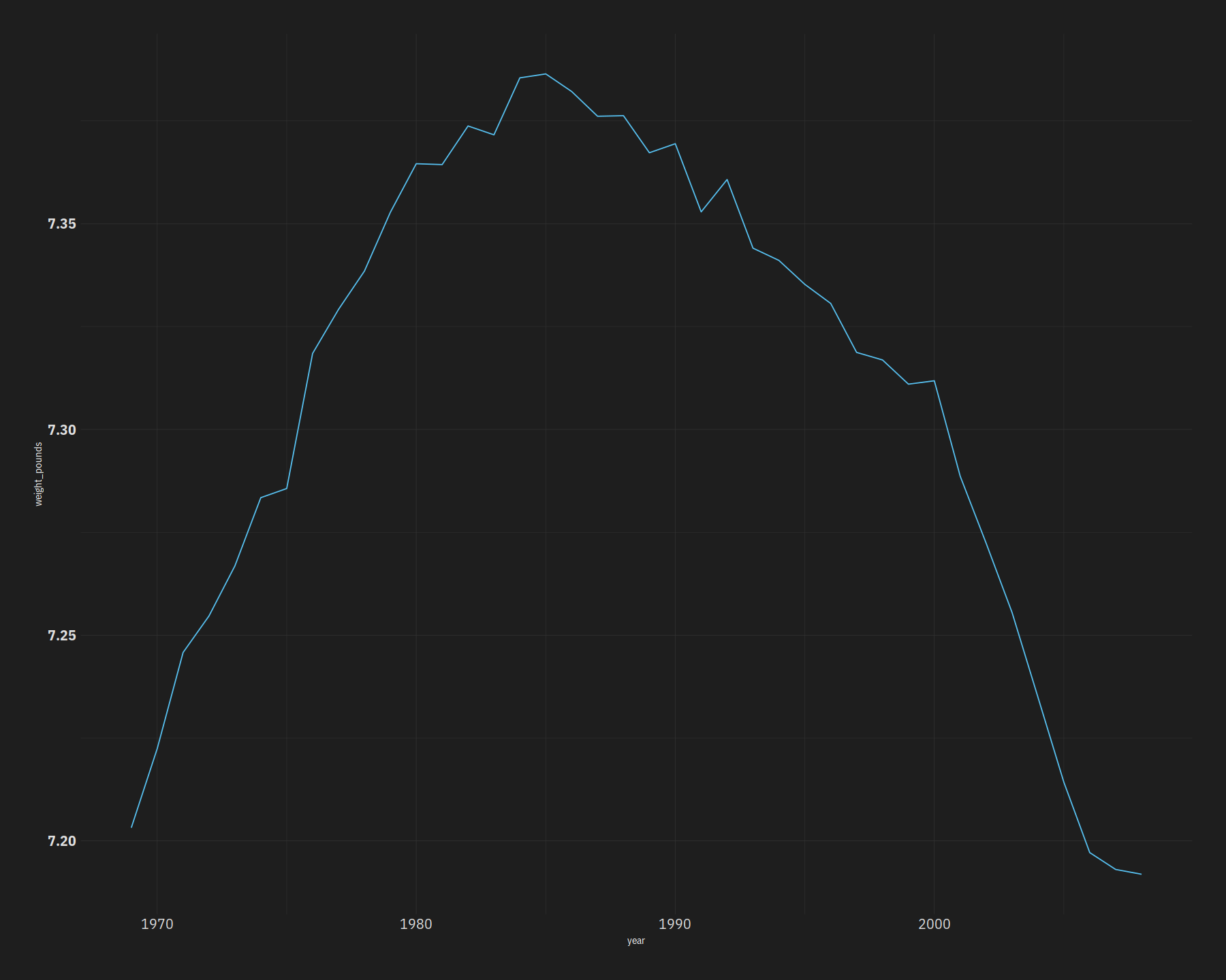
<BigQueryConnection>
  Dataset: publicdata.samples
  Billing: spatial-acumen-244921
  1. 'github_nested'
  2. 'github_timeline'
  3. 'gsod'
  4. 'natality'
  5. 'shakespeare'
  6. 'trigrams'
  7. 'wikipedia'

Natality

In [29]:
natality <- tbl(bq_con, "natality")
natality %>% glimpse
Rows: ??
Columns: 31
Database: BigQueryConnection
$ source_year            <int> 1969, 1969, 1970, 1970, 1970, 1970, 1971, 1971…
$ year                   <int> 1969, 1969, 1970, 1970, 1970, 1970, 1971, 1971…
$ month                  <int> 11, 2, 9, 1, 6, 10, 3, 8, 1, 5, 4, 9, 5, 9, 1,…
$ day                    <int> 29, 6, 4, 24, 6, 30, 18, 11, 23, 16, 15, 24, 3…
$ wday                   <int> NA, NA, NA, NA, NA, NA, NA, NA, NA, NA, NA, NA…
$ state                  <chr> "KS", "MN", "LA", "NC", "SC", "VA", "AZ", "CO"…
$ is_male                <lgl> TRUE, FALSE, TRUE, FALSE, TRUE, TRUE, FALSE, F…
$ child_race             <int> 1, 1, 1, 1, 2, 1, 1, 1, 2, 1, 1, 1, 1, 1, 2, 1…
$ weight_pounds          <dbl> 6.001, 8.938, 7.125, 7.626, 8.999, 6.499, 5.75…
$ plurality              <int> NA, NA, NA, NA, NA, NA, 1, 1, 1, NA, NA, NA, N…
$ apgar_1min             <int> NA, NA, NA, NA, NA, NA, NA, NA, NA, NA, NA, NA…
$ apgar_5min             <int> NA, NA, NA, NA, NA, NA, NA, NA, NA, NA, NA, NA…
$ mother_residence_state <chr> "KS", "MN", "LA", "NC", "SC", "VA", "AZ", "CO"…
$ mother_race            <int> 1, 1, 1, 1, 2, 1, 1, 1, 2, 1, 1, 1, 1, 1, 2, 1…
$ mother_age             <int> 20, 29, 29, 20, 18, 38, 26, 36, 19, 20, 27, 26…
$ gestation_weeks        <int> 36, 99, 40, 99, 31, NA, 41, 39, 37, 38, 40, NA…
$ lmp                    <chr> "03201999", "12991998", "11281999", "05991999"…
$ mother_married         <lgl> TRUE, TRUE, TRUE, TRUE, FALSE, TRUE, TRUE, TRU…
$ mother_birth_state     <chr> "", "", "LA", "NC", "SC", "VA", "IL", "SD", "I…
$ cigarette_use          <lgl> NA, NA, NA, NA, NA, NA, NA, NA, NA, NA, NA, NA…
$ cigarettes_per_day     <int> NA, NA, NA, NA, NA, NA, NA, NA, NA, NA, NA, NA…
$ alcohol_use            <lgl> NA, NA, NA, NA, NA, NA, NA, NA, NA, NA, NA, NA…
$ drinks_per_week        <int> NA, NA, NA, NA, NA, NA, NA, NA, NA, NA, NA, NA…
$ weight_gain_pounds     <int> NA, NA, NA, NA, NA, NA, NA, NA, NA, NA, NA, NA…
$ born_alive_alive       <int> 0, 2, 2, 0, 55, 0, 0, 5, 0, 0, 2, 1, 1, 1, 2, …
$ born_alive_dead        <int> 0, 0, 0, 0, 55, 0, 0, 0, 0, 0, 0, 0, 0, 0, 0, …
$ born_dead              <int> 0, 0, 0, 0, 55, 0, 0, 1, 0, 0, 0, 0, 0, 0, 0, …
$ ever_born              <int> 1, 3, 3, 1, 1, 1, 1, 7, 1, 1, 3, 2, 2, 2, 3, 1…
$ father_race            <int> 1, 1, 1, 1, 9, 1, 1, 1, 2, 1, 1, 1, 1, 1, 2, 1…
$ father_age             <int> 23, 28, 29, 21, 99, 36, 24, 37, 20, 23, 27, 26…
$ record_weight          <int> 2, 2, 2, 2, 2, 2, 2, 2, 2, 2, 2, 2, 2, 2, 2, 2…
In [30]:
bw <- natality %>%
  group_by(year) %>%
  summarise(weight_pounds = mean(weight_pounds, na.rm=T)) %>% 
  collect()

bw %>%
  ggplot(aes(year, weight_pounds)) + 
  geom_line()
Found more than one class "ident" in cache; using the first, from namespace 'dplyr'

Also defined by ‘dbplyr’

Found more than one class "ident" in cache; using the first, from namespace 'dplyr'

Also defined by ‘dbplyr’

In [37]:
dbDisconnect(bq_con)
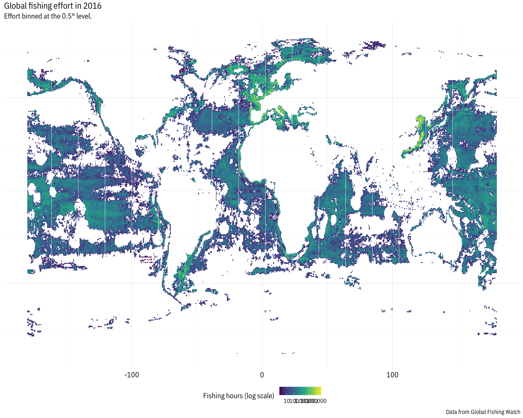
Fisheries

In [32]:
gfw_con <- 
  dbConnect(
    bigrquery::bigquery(),
    project = "global-fishing-watch",
    dataset = "global_footprint_of_fisheries",
    billing = projid
    )

dbListTables(gfw_con)
  1. 'fishing_effort'
  2. 'fishing_effort_byvessel'
  3. 'fishing_vessels'
  4. 'vessels'
In [33]:
effort <- tbl(gfw_con, "fishing_effort")
effort %>% glimpse
Rows: ??
Columns: 8
Database: BigQueryConnection
$ date          <chr> "2012-03-23", "2012-03-23", "2012-03-23", "2012-03-23",…
$ lat_bin       <int> -879, -5120, -5120, -5119, -5119, -5119, -5119, -5118, …
$ lon_bin       <int> 1324, -6859, -6854, -6858, -6854, -6855, -6853, -6852, …
$ flag          <chr> "AGO", "ARG", "ARG", "ARG", "ARG", "ARG", "ARG", "ARG",…
$ geartype      <chr> "purse_seines", "trawlers", "purse_seines", "purse_sein…
$ vessel_hours  <dbl> 5.7615, 1.5721, 3.0528, 2.4017, 1.5244, 0.7860, 4.6014,…
$ fishing_hours <dbl> 0.0000, 1.5721, 3.0528, 2.4017, 1.5244, 0.7860, 4.6014,…
$ mmsi_present  <int> 1, 1, 1, 1, 1, 1, 1, 1, 1, 1, 1, 1, 1, 1, 1, 1, 1, 1, 1…
In [36]:
effort %>%
  group_by(flag) %>%
  summarise(total_fishing_hours = sum(fishing_hours, na.rm=T)) %>%
  arrange(desc(total_fishing_hours)) %>%
  collect() %>% 
  head(10)
A tibble: 10 × 2
flagtotal_fishing_hours
<chr><dbl>
CHN57711389
ESP 8806223
ITA 6790417
FRA 6122613
RUS 5660001
KOR 5585248
TWN 5337054
GBR 4383738
JPN 4347252
NOR 4128516
In [39]:
## Define the desired bin resolution in degrees
resolution <- 0.5

effort %>%
  filter(
    `_PARTITIONTIME` >= "2016-01-01 00:00:00",
    `_PARTITIONTIME` <= "2016-12-31 00:00:00"
    ) %>%
  filter(fishing_hours > 0) %>%
  mutate(
    lat_bin = lat_bin/100,
    lon_bin = lon_bin/100
    ) %>%
  mutate(
    lat_bin_center = floor(lat_bin/resolution)*resolution + 0.5*resolution,
    lon_bin_center = floor(lon_bin/resolution)*resolution + 0.5*resolution
    ) %>%
  group_by(lat_bin_center, lon_bin_center) %>%
  summarise(fishing_hours = sum(fishing_hours, na.rm=T)) %>%
  collect() -> 
    globe
In [41]:
globe %>% 
  filter(fishing_hours > 1) %>% 
  ggplot() +
  geom_tile(aes(x=lon_bin_center, y=lat_bin_center, fill=fishing_hours))+
  scale_fill_viridis_c(
    name = "Fishing hours (log scale)",
    trans = "log",
    breaks = scales::log_breaks(n = 5, base = 10),
    labels = scales::comma
    ) +
  labs(
    title = "Global fishing effort in 2016",
    subtitle = paste0("Effort binned at the ", resolution, "° level."),
    y = NULL, x = NULL,
    caption = "Data from Global Fishing Watch"
    ) +
  lal_plot_theme() +
  theme(axis.text=element_blank())
In [42]:
dbDisconnect(gfw_con)