Regularized Estimators and scikit-learn Comparison

This notebook demonstrates the new regularized estimator API in pyensmallen. When alpha > 0, the linear, logistic, and Poisson estimator classes switch from unconstrained L_BFGS to exact Frank-Wolfe optimization over either an L2 ball (l1_ratio=0.0) or an L1 ball (l1_ratio=1.0).

The second half of the notebook compares pyensmallen with scikit-learn on a moderate p versus n linear problem and plots out-of-sample MSE over a grid of regularization strengths.

import os
import sys
import warnings

candidate_roots = [
    os.getcwd(),
    os.path.abspath(".."),
    os.path.abspath(os.path.join("..", "..")),
]
repo_root = next(
    path
    for path in candidate_roots
    if os.path.exists(os.path.join(path, "pyensmallen", "__init__.py"))
)
if repo_root not in sys.path:
    sys.path.insert(0, repo_root)

sys.meta_path = [
    finder
    for finder in sys.meta_path
    if getattr(finder.__class__, "__module__", "") != "_pyensmallen_editable_loader"
]

warnings.filterwarnings("ignore", message=".*joblib will operate in serial mode.*")
warnings.filterwarnings("ignore", category=FutureWarning, module="sklearn")

import matplotlib.pyplot as plt
import numpy as np
import pandas as pd
import seaborn as sns
from scipy.special import expit
from sklearn.linear_model import Lasso, LogisticRegression as SkLogit, PoissonRegressor, Ridge
from sklearn.metrics import (
    accuracy_score,
    log_loss,
    mean_poisson_deviance,
    mean_squared_error,
)

import pyensmallen as pe

sns.set_theme(style="whitegrid")
rng = np.random.default_rng(12345)

Shared regularization API across estimators

All three estimator classes accept the same regularization arguments:

• alpha=0.0 keeps the unregularized L_BFGS fit
• alpha>0, l1_ratio=0.0 uses Frank-Wolfe over an L2 ball
• alpha>0, l1_ratio=1.0 uses Frank-Wolfe over an L1 ball

Below we fit one regularized example for each estimator class and compare it with the closest scikit-learn counterpart using a common metric.

rows = []

# Linear regression: compare against scikit-learn Lasso.
n_linear, p_linear = 600, 12
X_linear = rng.normal(size=(n_linear, p_linear))
beta_linear = np.zeros(p_linear)
beta_linear[:4] = np.array([1.0, -0.75, 0.5, 0.25])
y_linear = 0.4 + X_linear @ beta_linear + rng.normal(scale=0.7, size=n_linear)

alpha_linear = 0.5
py_linear = pe.LinearRegression(alpha=alpha_linear, l1_ratio=1.0).fit(X_linear, y_linear)
sk_linear = Lasso(alpha=alpha_linear, fit_intercept=True, max_iter=10000, tol=1e-6).fit(X_linear, y_linear)

for library, model in [("pyensmallen", py_linear), ("scikit-learn", sk_linear)]:
    rows.append(
        {
            "estimator": "LinearRegression",
            "library": library,
            "regularization": "L1",
            "metric": "train MSE",
            "value": mean_squared_error(y_linear, model.predict(X_linear)),
            "coef_norm": np.linalg.norm(model.coef_, 1),
            "optimizer": getattr(model, "optimizer_name_", "coordinate descent"),
        }
    )

# Logistic regression: compare against scikit-learn's l2-regularized logit.
X_logit = rng.normal(size=(800, 3))
eta = -0.3 + X_logit @ np.array([1.2, -0.9, 0.6])
p_logit = expit(eta)
y_logit = rng.binomial(1, p_logit)

alpha_logit = 0.25
py_logit = pe.LogisticRegression(alpha=alpha_logit, l1_ratio=0.0).fit(X_logit, y_logit)
sk_logit = SkLogit(C=1.0 / alpha_logit, solver="lbfgs", fit_intercept=True, max_iter=5000).fit(X_logit, y_logit)

for library, model, probs in [
    ("pyensmallen", py_logit, py_logit.predict_proba(X_logit)[:, 1]),
    ("scikit-learn", sk_logit, sk_logit.predict_proba(X_logit)[:, 1]),
]:
    rows.append(
        {
            "estimator": "LogisticRegression",
            "library": library,
            "regularization": "L2",
            "metric": "log loss",
            "value": log_loss(y_logit, probs),
            "coef_norm": np.linalg.norm(model.coef_),
            "optimizer": getattr(model, "optimizer_name_", "lbfgs"),
        }
    )
    rows.append(
        {
            "estimator": "LogisticRegression",
            "library": library,
            "regularization": "L2",
            "metric": "accuracy",
            "value": accuracy_score(y_logit, (probs >= 0.5).astype(int)),
            "coef_norm": np.linalg.norm(model.coef_),
            "optimizer": getattr(model, "optimizer_name_", "lbfgs"),
        }
    )

# Poisson regression: compare against scikit-learn PoissonRegressor.
X_pois = rng.normal(size=(800, 3))
mu = np.exp(0.2 + X_pois @ np.array([0.3, -0.2, 0.15]))
y_pois = rng.poisson(mu)

alpha_pois = 0.25
py_pois = pe.PoissonRegression(alpha=alpha_pois, l1_ratio=0.0).fit(X_pois, y_pois)
sk_pois = PoissonRegressor(alpha=alpha_pois, fit_intercept=True, max_iter=5000).fit(X_pois, y_pois)

for library, model, preds in [
    ("pyensmallen", py_pois, py_pois.predict(X_pois)),
    ("scikit-learn", sk_pois, sk_pois.predict(X_pois)),
]:
    rows.append(
        {
            "estimator": "PoissonRegression",
            "library": library,
            "regularization": "L2",
            "metric": "mean Poisson deviance",
            "value": mean_poisson_deviance(y_pois, np.clip(preds, 1e-8, None)),
            "coef_norm": np.linalg.norm(model.coef_),
            "optimizer": getattr(model, "optimizer_name_", "lbfgs"),
        }
    )

shared_api_results = pd.DataFrame(rows)
shared_api_results

	estimator	library	regularization	metric	value	coef_norm	optimizer
0	LinearRegression	pyensmallen	L1	train MSE	0.660204	1.828547	FrankWolfe
1	LinearRegression	scikit-learn	L1	train MSE	1.336264	0.748089	coordinate descent
2	LogisticRegression	pyensmallen	L2	log loss	0.498372	1.621752	FrankWolfe
3	LogisticRegression	pyensmallen	L2	accuracy	0.765000	1.621752	FrankWolfe
4	LogisticRegression	scikit-learn	L2	log loss	0.498372	1.618707	lbfgs
5	LogisticRegression	scikit-learn	L2	accuracy	0.765000	1.618707	lbfgs
6	PoissonRegression	pyensmallen	L2	mean Poisson deviance	1.174252	0.432143	FrankWolfe
7	PoissonRegression	scikit-learn	L2	mean Poisson deviance	1.180530	0.359993	lbfgs

Moderate p versus n: out-of-sample MSE path

We now generate a sparse linear problem with p=120 features and only n=200 training observations. The goal is not to numerically match scikit-learn’s penalty parameterization exactly. Instead, the same grid of regularization strengths is used in both libraries so we can compare the shape of the MSE path and the best achievable out-of-sample error.

Two comparisons are shown:

• pyensmallen L2-constrained fit vs scikit-learn Ridge
• pyensmallen L1-constrained fit vs scikit-learn Lasso

n_train, n_test, p = 200, 2000, 120
n_active = 12
alpha_grid = np.logspace(-2, 1.2, 12)

X_train = rng.normal(size=(n_train, p))
X_test = rng.normal(size=(n_test, p))

beta_true = np.zeros(p)
active = rng.choice(p, size=n_active, replace=False)
beta_true[active] = rng.normal(loc=0.0, scale=1.5, size=n_active)
intercept_true = 0.5

y_train = intercept_true + X_train @ beta_true + rng.normal(scale=1.0, size=n_train)
y_test = intercept_true + X_test @ beta_true + rng.normal(scale=1.0, size=n_test)

print(f"train shape: {X_train.shape}, test shape: {X_test.shape}")
print(f"nonzero coefficients: {n_active}")

train shape: (200, 120), test shape: (2000, 120)
nonzero coefficients: 12

rows = []

for alpha in alpha_grid:
    py_l2 = pe.LinearRegression(alpha=float(alpha), l1_ratio=0.0).fit(X_train, y_train)
    py_l1 = pe.LinearRegression(alpha=float(alpha), l1_ratio=1.0).fit(X_train, y_train)
    sk_ridge = Ridge(alpha=float(alpha), fit_intercept=True).fit(X_train, y_train)
    sk_lasso = Lasso(alpha=float(alpha), fit_intercept=True, max_iter=10000, tol=1e-6).fit(X_train, y_train)

    for model_name, model, penalty in [
        ("pyensmallen-l2", py_l2, "l2"),
        ("pyensmallen-l1", py_l1, "l1"),
        ("sklearn-ridge", sk_ridge, "l2"),
        ("sklearn-lasso", sk_lasso, "l1"),
    ]:
        rows.append(
            {
                "alpha": alpha,
                "model": model_name,
                "penalty": penalty,
                "train_mse": mean_squared_error(y_train, model.predict(X_train)),
                "test_mse": mean_squared_error(y_test, model.predict(X_test)),
                "coef_l1": np.linalg.norm(model.coef_, 1),
                "coef_l2": np.linalg.norm(model.coef_, 2),
            }
        )

results = pd.DataFrame(rows)
results.head()

	alpha	model	penalty	train_mse	test_mse	coef_l1	coef_l2
0	0.010000	pyensmallen-l2	l2	0.300465	2.424340	26.118816	5.381626
1	0.010000	pyensmallen-l1	l1	0.578212	1.615896	19.914086	5.318775
2	0.010000	sklearn-ridge	l2	0.297860	2.427721	26.179356	5.403925
3	0.010000	sklearn-lasso	l1	0.331483	1.656856	22.333471	5.330794
4	0.019539	pyensmallen-l2	l2	0.298860	2.423294	26.105470	5.379762

best_by_model = (
    results.sort_values("test_mse")
    .groupby("model", as_index=False)
    .first()[["model", "alpha", "train_mse", "test_mse", "coef_l1", "coef_l2"]]
    .sort_values("test_mse")
)
best_by_model

	model	alpha	train_mse	test_mse	coef_l1	coef_l2
2	sklearn-lasso	0.074598	0.662303	1.202322	17.055005	5.084258
0	pyensmallen-l1	0.010000	0.578212	1.615896	19.914086	5.318775
3	sklearn-ridge	1.087336	0.300220	2.418005	25.950701	5.322411
1	pyensmallen-l2	0.145759	0.298654	2.419524	26.050077	5.358361

fig, axes = plt.subplots(1, 2, figsize=(13, 4.5), sharey=True)

curve_specs = [
    ("l2", [("pyensmallen-l2", "pyensmallen", "o"), ("sklearn-ridge", "scikit-learn", "s")], "L2 regularization"),
    ("l1", [("pyensmallen-l1", "pyensmallen", "o"), ("sklearn-lasso", "scikit-learn", "s")], "L1 regularization"),
]

for ax, (penalty, curves, title) in zip(axes, curve_specs):
    panel = results.loc[results["penalty"] == penalty]
    for model_name, label, marker in curves:
        curve = panel.loc[panel["model"] == model_name].sort_values("alpha")
        ax.plot(
            curve["alpha"],
            curve["test_mse"],
            marker=marker,
            linewidth=2,
            label=label,
        )
    ax.set_xscale("log")
    ax.set_title(title)
    ax.set_xlabel("regularization strength")
    ax.grid(True, alpha=0.3)

axes[0].set_ylabel("test MSE")
axes[0].legend(frameon=True)
axes[1].legend(frameon=True)
fig.suptitle("Out-of-sample MSE path on a sparse moderate-p/n problem", y=1.03)
fig.tight_layout()
plt.show()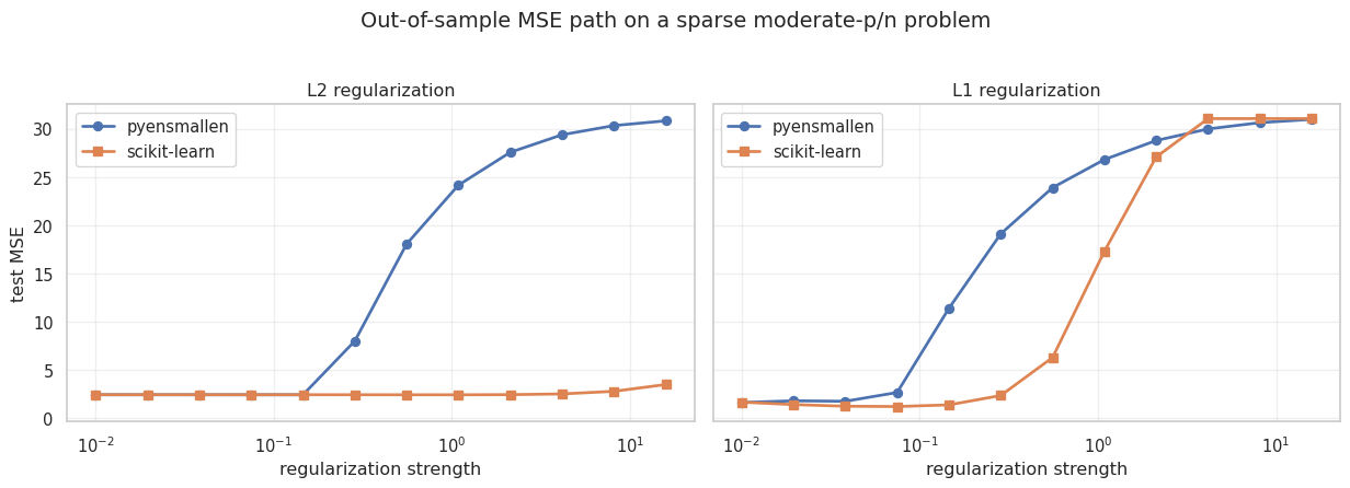

Takeaways

• The same estimator interface now covers unregularized and exact constrained regularized fits.
• The regularized pyensmallen fits quietly switch to Frank-Wolfe on the backend.
• On this sparse moderate-p problem, the L1 path is much more competitive than the L2 path, which is what we would expect.
• The MSE curves have the same broad shape as the scikit-learn baselines, even though the two libraries do not use identical regularization parameterizations.