Chapter 04: Maximum Likelihood and Machine Learning

This note is a high-fidelity Markdown migration of the Maximum Likelihood and Machine Learning chapter from the LaTeX source.

Parent map: index Prerequisites: probability-and-mathstats, linear-regression, causal-inference

Concept map

flowchart TD
  A[Maximum Likelihood] --> B[Score / Fisher Information]
  A --> C[QMLE / Robust SEs]
  A --> D[Binary / Discrete Choice]
  D --> E[Ordered / Unordered Models]
  A --> F[Counts / Rates / Truncation]
  A --> G[GLM Theory]
  H[Machine Learning] --> I[Supervised Learning]
  I --> J[Regularization]
  I --> K[Classification Metrics]
  H --> L[Neural Networks]
  H --> M[Unsupervised Learning]

Maximum Likelihood

Setup

Let $\{Z{\}}_{i=1}^N$ be a sequence of iid rv’s with common CDF $F(z|{\theta }^{\ast })$. We want to estimate ${\theta }^{\ast }\in \Theta \subset {\mathbb{R}}^k$.

Since the rv’s are IID, we can write

$$f(\mathbf{y}|{\theta }^{\ast })=\prod _{i=1}^{N}f(y_i|{\theta }^{\ast })$$

L: $\Theta \to \mathbb{R}$

$$L(\theta |\mathbf{y}):=\prod _{i=1}^{N}f(y_i|\theta )$$

We usually work with the log of this $\ell (\theta |y):={\sum }_{i=1}^N\log f(y_i|\theta )$, and drop the conditioning on $y$ though strictly speaking $f(\mathbf{y},\mathbf{X}|\theta )=f(\mathbf{y}|\mathbf{X}|\theta )f(\mathbf{X}|\theta )$

is the estimator that maximises the conditional log-likelihood estimator.

$${\hat{\theta }}_{MLE}:=\underset{\theta \in \Theta }{\mathrm{argmax}}\mathcal{L}(\theta )=\underset{\theta \in \Theta }{\mathrm{argmax}}\sum _{i=1}\log f(Z_i|\theta )$$

solves the first-order conditions

$$\frac{1}{N}\frac{\partial \mathcal{L}(\theta )}{\partial \theta }=\frac{1}{N}\sum _i\frac{\partial \ell (y_i|x_i,\theta )}{\partial \theta }=0$$

conditional density:

$$f(y_i|x_i,|\beta ,{\sigma }^2)=\prod _{i=1}^N\frac{1}{\sqrt{2\pi {\sigma }^2}}\exp \left(-\frac{(y_i-x_i^{\prime }\beta {)}^2}{2{\sigma }^2}\right)$$

Log likelihood:

$$\begin{array}{rl}\ell (\beta ,{\sigma }^2)& =-\frac{n}{2}\log (2\pi )-\frac{n}{2}\log {\sigma }^2-\frac{1}{2{\sigma }^2}(y-X\beta {)}^{\prime }(y-X\beta )\\ & =-\frac{N}{2}\mathbf{RSS}(\beta )-\frac{N}{2}\log (2\pi {\sigma }^2)\end{array}$$

Maximising this w.r.t. $b,s^2$ yields $\hat{\beta }={\left(X^{\prime }X\right)}^{-1}{X}^{\prime }y$, ${\hat{\sigma }}^2=\frac{{\sum }_{i=1}^n{\hat{u}}_i^2}{N}$.

gradient vector $\mathcal{S}(\theta ):=\nabla \ell (\theta )=\frac{\partial \ell (\theta )}{\partial \theta }$

$$\mathcal{S}(z,\theta ):=\frac{\partial \ell (\theta )}{\partial \theta }(z;\theta )$$

Evaluated at ${\theta }^{\ast }$, this is the efficient score.

local maximum that solves the FOCs $\mathcal{S}(z,\theta )=0$, IOW

$$\frac{1}{N}\sum _{i=1}^N\frac{\log f(Z_i|\theta )}{\partial \theta }=0$$ $$\mathcal{I}(\theta ):=\mathbb{E}\left[\mathcal{S}(\theta )\mathcal{S}(\theta {)}^{\prime }\right]=\mathbb{E}\left[\frac{\partial \ell (\theta )}{\partial \theta }\frac{\partial \ell (\theta )}{\partial {\theta }^{\prime }}\right]=-\mathbb{E}\left[\frac{{\partial }^2\ell (\theta )}{\partial \theta \partial {\theta }^{\prime }}\right]$$ $$\mathcal{A}=\mathcal{B}:=\mathbb{V}\left[s_i({\theta }^{\ast })\right]=\mathbb{E}\left[s_i({\theta }^{\ast })s_i({\theta }^{\ast }{)}^{\prime }\right]=\mathbb{E}\left[\frac{\partial }{\partial \theta }{s}_i({\theta }^{\ast })\right]$$

Variance estimate $\mathbb{V}\left[\hat{\theta }\right]=\frac{1}{n}{\mathcal{A}}^{-1}$;

Estimated as

$$\widehat{\mathcal{I}(\theta )}=-\frac{1}{N}\sum _{i=1}^N{\frac{{\partial }^2{\ell }_i(\theta )}{\partial \theta \partial {\theta }^{\prime }}|}_{\theta ={\theta }_{MLE}}$$

For OLS, parameter vector $\theta =({\beta }^{\prime },{\sigma }^2{)}^{\prime })=({\beta }^{\prime },\gamma {)}^{\prime }$.

Scores:

$$\frac{\partial \ell }{\partial \beta }=\frac{1}{\gamma }{X}^{\prime }(y-X\beta )$$ $$\begin{array}{rl}\frac{\partial \ell }{\partial \gamma }& =-\frac{n}{2\gamma }+\frac{1}{2{\gamma }^2}\underset{:=s}{\underbrace{(y-X\beta {)}^{\prime }(y-x\beta )}}\\ \gamma & =s/n=\frac{1}{n}\sum _{i=1}^n(y_i-{\mathbf{x}}_i^{\prime }\beta )\end{array}$$

Information Matrix / Variance

$$I(\theta )=\left(\begin{array}{cc}\frac{1}{{\sigma }^2}{X}^{\prime }X& 0\\ 0^{\prime }& \frac{n}{2{\sigma }^4}\end{array}\right)⟹CRLB:={\left(I(\theta )\right)}^{-1}=\left(\begin{array}{cc}{\sigma }^2{\left(X^{\prime }X\right)}^{-1}& 0\\ 0^{\prime }& \frac{2{\sigma }^4}{n}\end{array}\right)$$

Properties of Maximum Likelihood Estimators

$N\to \infty$, probability of missing the true parameter goes to zero.

$$P(|{\hat{\theta }}_n-\theta |>ϵ)\stackrel{p}{\to }0\forall ϵ>0$$ $$\sqrt{N}(\hat{\theta }-\theta )\stackrel{d}{\to }\mathcal{N}(0,\mathcal{I}(\theta {)}^{-1})$$

Equivalently,

$${\hat{\theta }}_{MLE}{\sim }^a\mathcal{N}\left(\theta ,-\mathbb{E}{\left[\frac{{\partial }^2\ell (\theta )}{\partial \theta \partial {\theta }^{\prime }}\right]}^{-1}\right)$$

conditions: (1) $\theta \in \Theta$ , (2) $\ell$ is twice-differentiable Variance of MLE is the Cramer-Rao Bound; the asymptotic variance of the MLE is at least as small as that of any other consistent estimator. Let the pdf of the r.v. $X$ be $f_X(x|\theta )$ for some ${\theta }_0\in \Theta$. Let $\hat{\theta }$ be an unbiased estimator for ${\theta }_0$. Suppose the derivative $\partial /\partial \theta$ can be passed under the integral $\int f(x|\theta )dx$ and $\int \theta (x)f(x|\theta )dx$ and suppose the fisher information

$$\mathcal{I}(\theta )=-\mathbb{E}\left[\frac{{\partial }^2\log f}{\partial \theta \partial {\theta }^{\prime }}(X|\theta )\right]$$

is finite. Then,

$$\mathbb{V}\left[\hat{\theta }(X)\right]\ge \mathcal{I}({\theta }_0{)}^{-1}$$

If $X_1,X_2,\dots ,X_n$ are iid with common density ${\mathsf{f}}_x(x|\theta )$, the implied bound on the variance is $N\mathbb{V}\left[\hat{\theta }(X)\right]\ge \mathcal{I}({\theta }_0{)}^{-1}$ Let $X_1,X_2,\dots$ be iid random variables with common density ${\mathsf{f}}_x(x|\theta )$. A sequence of estimates ${\hat{\theta }}_N$, a function $X_1,X2,\dots ,X_N$ that satisfies

$$\sqrt{N}({\hat{\theta }}_{ml}-\theta )\stackrel{d}{\to }\mathcal{N}\left(0,\mathcal{I}(\theta {)}^{-1}\right)$$

whatever the true value of $\theta \in \Theta$ is, is said to be asymptotically efficient. Suppose $X_1,X_2,\dots$ are iid with density $X\sim f(x|\theta ,h(.))$ where $h(.)$ is an unknown function. Next, we pretend to know the infinite dimensional parameter $h()$ up to a finite dimensional parameter $\gamma$, in which we have a fully parametric finite-dimensional parameter $\theta$, thus we can calculate the Cramer-Rao Bound.

$$f(x|\theta ,\gamma )=f(x|\theta ,h(\gamma ))$$

Partitioning the information matrix for $({\theta }^{\prime },{\gamma }^{\prime }{)}^{\prime }$ and its inverse in

$$\mathcal{I}(\theta ,\gamma )=\left[\begin{array}{cc}{\mathcal{I}}_{\theta {\theta }^{\prime }}& {\mathcal{I}}_{\theta {\gamma }^{\prime }}\\ {\mathcal{I}}_{{\gamma }^{\prime }\theta }& {\mathcal{I}}_{\gamma {\gamma }^{\prime }}\end{array}\right]\text{and }\mathcal{I}(\theta ,\gamma {)}^{-1}=\left[\begin{array}{cc}{\mathcal{I}}^{\theta {\theta }^{\prime }}& {\mathcal{I}}^{\theta {\gamma }^{\prime }}\\ {\mathcal{I}}^{\gamma {\theta }^{\prime }}& {\mathcal{I}}^{\gamma {\gamma }^{\prime }}\end{array}\right]$$

The Cramer-Rao bound implies that

$$ASV(\hat{\theta })\ge {\mathcal{I}}^{\theta {\theta }^{\prime }}=({\mathcal{I}}_{\theta {\theta }^{\prime }}-{\mathcal{I}}_{\theta {\gamma }^{\prime }}{\left({\mathcal{I}}_{\gamma {\gamma }^{\prime }}\right)}^{-1}{\mathcal{I}}_{\gamma {\theta }^{\prime }}{)}^{-1}$$

This is true for any parametrisation of the unknown function $h(.)$. The lowest possible variance for any estimator for $\theta$ that does not use knowledge of $h(.)$ has to be at least as high as the lowest variance we can get if we know more, that is, the Cramer-Rao bound for any parametric submodel. So, the semiparametric efficiency bound is the largest lower-bound we can get for any parametric submodel.

Suppose we have a candidate Estimator $\hat{\theta }$ and a given parametrisation $h(x;\gamma )$. Then,

$$({\mathcal{I}}_{\theta {\theta }^{\prime }}-{\mathcal{I}}_{\theta {\gamma }^{\prime }}{\left({\mathcal{I}}_{\gamma {\gamma }^{\prime }}\right)}^{-1}{\mathcal{I}}_{\gamma {\theta }^{\prime }}{)}^{-1}\le \text{Semiparametric Efficiency Bound}\le ASV(\hat{\theta })$$

For any estimator we can calculate the left hand side, for any parametrization we can calculate the right hand side, so if we find an estimator and a parametrization that the two are equal we have found the efficiency bound. Let $\tau =g(\theta )$ where $g$ is bijective, continuous, and differentiable. Let ${\hat{\theta }}_n$ be the MLE of $\theta$. Then, ${\hat{\tau }}_n=g(\widehat{{\theta }_n}$ is the MLE of $\tau$. For a regression of the form $\mathbb{E}\left[y|x\right]=g(x^{\prime }\beta )$, one can estimate multiple ‘marginal effects’. For the special case where $\mathbb{E}\left[y|x\right]=x^{\prime }\beta$, $\frac{\partial \mathbb{E}\left[y|x\right]}{\partial x}=\beta$, but this is not generically true.

Average Marginal Effect (AME): $:=\frac{1}{N}{\sum }_i\frac{\partial \mathbb{E}\left[y_i|x_i\right]}{\partial x_i}$

Marginal Effect at Mean (MEM) $\frac{\partial \mathbb{E}\left[y|x\right]}{\partial x}{|}_{\bar{x}}$ Suppose $t(x)$ is a sufficient statistic for $\theta$. Then,

$$\prod _{i}f(x_i|\theta )=g\left(t(x),\theta \right)h(x)$$

$\hat{\theta }(x)$ depends on the data $x$ only through $t(x)$, the sufficient statistic.

QMLE / Misspecification / Information Theory

If model is misspecified, $f\left(\cdot |x_i,\theta \right)\ne p_0\left(\cdot |x_i\right)\forall \theta \in \Theta$

The MLE converges to the best fitting $\theta$ for the population (pseudo-true value)

$$\begin{array}{rl}{\theta }^{\star }& =\underset{\theta \in \Theta }{\mathrm{argmax}}\mathrm{plim}\frac{1}{N}\sum _{i=1}^N{\ell }_i(\theta )\end{array}$$

For the linear exponential family, the quasi-MLE is consistent even when the density is partially misspecified.

Robust Standard Errors

Asymptotic distribution of QMLE

$$\sqrt{n}\left(\hat{\theta }-{\theta }^{\star }\right)\stackrel{d}{\to }\mathcal{N}\left(0,{\hat{A}}^{-1}\hat{B}{\hat{A}}^{-1}\right)$$

where

$$\hat{A}=-\mathbb{E}\left[{\nabla }^2(\hat{\beta })\right]=\mathbb{E}\left[\frac{\partial {\mathcal{S}}_i(\theta )}{\partial {\theta }^{\prime }}\right]{|}_{\hat{\theta }}=\frac{1}{n}\sum _{i=1}^n\frac{{\partial }^2{\ell }_i(\theta )}{\partial \theta \partial {\theta }^{\prime }}{|}_{\hat{\theta }}$$ $$\hat{B}=\mathbb{E}\left[{\mathcal{S}}_i\left({\theta }^{\star }\right){\mathcal{S}}_i{\left({\theta }^{\star }\right)}^{\prime }\right]=\frac{1}{n}\sum _{i=1}^n\frac{\partial {\ell }_i}{\partial \theta }\times \frac{\partial {\ell }_i}{\partial {\theta }^{\prime }}{|}_{\hat{\theta }}$$

let $f(y|\theta )$ be the assumed joint density, and let $h(y)$ be the true density. Then,

$$\text{KL}[h(\cdot )||f(\cdot )]:={\mathbb{E}}_h\left[\log \left(\frac{h(y)}{f(y|\theta )}\right)\right]={\int }_{-\infty }^{\infty }h(t)\log \left(\frac{h(t)}{f(t)}\right)dt$$

Minimised when $\exists {\theta }_0\text{ s.t. }h(y)=f(y|{\theta }_0)$. QMLE minimises distance between $f(y|\theta )$ and $h(y)$. Notation $\text{KL}(h,f)$ denotes ‘information lost when $f$ is used to approximate $h$‘.

Discrete version illustrates links to Entropy

$$\text{KL}[p||q]:=\sum _{j=1}^J{p}_j\log \frac{p_j}{q_j}=\sum _{j=1}^J{p}_j\log p_j-\sum _{j=1}^J{p}_j\log q_j=-\mathbb{H}(p)+\underset{\text{cross entropy}}{\underbrace{\mathbb{H}(p,q)}}$$

$KL(p||q)\ge 0$ and with equality IFF $p=q$.

$KL$ ‘distance’, unlike Euclidian Distance, is not the same between $f,g$ as $g,f$; i.e. it is directional. Akaike showed that using K-L model selection entails finding a good estimator for

$${\mathbb{E}}_{y,h}\left[{\mathbb{E}}_{x,h}\left[\log (f(x|\hat{\theta }(y)))\right]\right]$$

where $x,y$ are independent, random samples from the same distribution and expectations are taken w.r.t. the true distribution $h$. Estimating this quantity for each model ${\mathfrak{f}}_i$ is biased upwards. An approximately unbiased estimator of the above target quantity is

For a general class of maximum-likelihood models,

$$\text{AIC}=-2\log \mathcal{L}(\hat{\mathbf{\theta }}|\mathbf{y})+2K$$

For linear regression models, this simplifies to

$$AIC=n\log {\hat{\sigma }}^2+2K;{\hat{\sigma }}^2=\frac{{\sum }_{i=1}^n{\hat{\epsilon }}^2}{n}$$ $$BIC=\ln \left(\frac{e^{\prime }e}{n}\right)+\frac{k\ln (n)}{n}$$

Testing

To test the hypothesis $H_0:\alpha =0$ against the alternative, there are three classical tests.

We partition the parameter $K$-vector $\theta$ into two parts $({\theta }_0^{\prime },{\theta }_1^{\prime }{)}^{\prime }$ s.t. the dimensions of the two sub-vectors s.t. $K_0+K_1=K$. ${\theta }_1$ is a nuisance parameter: its value is not restricted under the null.

Let ${\hat{\theta }}_u:=({\hat{\theta }}_{0u},{\hat{\theta }}_{1u})$ be the unrestricted MLEs. If we are testing the restriction ${\theta }_0=0$, then the restricted parameter vector is ${\hat{\theta }}_R:=(0,{\hat{\theta }}_{1r})$. IOW, test $\mathbf{h}({\theta }_0)=0$.

If null is true, $\ell$ at restricted model ($(0,{\theta }_{1r}$) should not be much smaller than $\ell$ at the unrestricted model ($({\theta }_{0u},{\theta }_{1u})$.

$$LR:=2\times (\ell ({\hat{\theta }}_u)-\ell ({\hat{\theta }}_R))$$

Under the null, $LR\sim {\chi }_{K_0}^2$ (where $K_0$ is the number of restrictions being tested). If the limiting $\ell$ is maximised at ${\theta }_0=0$, the derivative of the $\ell$ wrt ${\theta }_0$ at that point should be close to zero.

$$LM:=\mathcal{S}({\hat{\theta }}_R{)}^{\prime }[{\mathcal{I}}^{-1}({\hat{\theta }}_R)]\mathcal{S}({\hat{\theta }}_R)$$

Under the null, $LR\sim {\chi }_{K_0}^2$ (where $K_0$ is the number of restrictions being tested). Unrestricted estimates of ${\theta }_0$ should be close to zero.

$$W:=N\cdot {\hat{\theta }}_{0u}^{\prime }{\left({\hat{\mathcal{I}}}^{00}\right)}^{-1}{\hat{\theta }}_{0u}$$

Where ${\hat{\mathcal{I}}}^{00}$ is the top-left of the information matrix (corresponding with the restricted parameters). Under the null, $W\sim {\chi }_{K_0}^2$.

alternatively, $W=h({\hat{\theta }}_u{)}^{\prime }{\Omega }^{-1}h({\hat{\theta }}_u)$

where $h_1(\theta )\dots h_{K_0}(\theta )$ are restrictions,

$$\Omega ={\left(\frac{\partial h(\theta )}{\partial \theta }\right)}^{\prime }\mathbb{V}\left[{\theta }_u\right]\left(\frac{\partial h(\theta )}{\partial \theta }\right)$$

evaluated at ${\hat{\theta }}_u$. McFadden’s Pseudo-$R^2$

$$R_{bin}^2:=1-\frac{\ell (\hat{\beta })}{\ell (\bar{y})}$$

Binary Choice

Estimate the probability using OLS $\mathbf{Pr}\left(y=1|\mathbf{x}\right)=\mathbf{X}\mathbf{\beta }$. $\mathbb{V}\left[y|\mathbf{x}\right]=\mathbf{X}\mathbf{\beta }(1-\mathbf{X}\mathbf{\beta })$, so heteroskedasticity is mechanically present unless all coefficients are zero.

$$\text{Logit(p)}=\log \left(\frac{p}{1-p}\right)$$ $$\text{Logistic(x)}=\frac{1}{1+\exp (-x)}=\frac{e^x}{1+e^x}$$

Logistic regression fits $\text{logit}(p_i)=x_i^{\prime }\beta$, where $logit$ is the link function that scales $x_i^{\prime }\beta$ onto the probability scale. Alternatively, one can use $\Phi (0,1)$. For $Y_i\in \{0,1\}$, assume latent index model $Y_i^* = X_i’\beta

• \epsilon_i$;$Y_i \defeq \Indic{Y_i^* > 0}$.$Y_i$isbernoulli,so$\mathcal{L}=\prod_{i=1}^{N} \pi_{i}^{Y_{i}}\left(1-\pi_{i}\right)^{1-Y_{i}}$.

Symmetric CDFs. Let ${\pi }_i=\mathbb{E}\left[Y_i|X_i\right]=\mathbf{Pr}\left(Y_i=1|X_i\right)=\mathbb{F}(X_i^{\prime }\beta )=1-\mathbb{F}(-X_i^{\prime }\beta )$

Probit: $\mathbb{F}(u)=\Phi (u)$

Logit:

$\mathbb{F}(u)=\Lambda (u)$ = $\frac{1}{1+\exp (-u)}=\frac{\exp (u)}{1+\exp (u)}$

$f(u)={\Lambda }^{\prime }(u)=(1-e^{-u}{)}^{-2}{e}^{-u}$

Model	${\pi }_i=\mathbf{Pr}\left(y=1\mid x\right)$	Marginal Effect $\frac{\partial p}{\partial x_j}$
Logit	$\Lambda (x^{\prime }\beta )=\frac{\exp (x^{\prime }\beta )}{1+\exp (x^{\prime }\beta )}$	$\Lambda (x^{\prime }\beta )\left[1-\Lambda (x^{\prime }\beta )\right]{\beta }_j$
Probit	$\Phi (x^{\prime }\beta )$	$\varphi (x^{\prime }\beta ){\beta }_j$
Clog-log	$C(x^{\prime }\beta )=1-\exp (-\exp (x^{\prime }\beta ))$	$\exp (-\exp (x^{\prime }\beta ))\exp (x^{\prime }\beta ){\beta }_j$
LPM	$x^{\prime }\beta$	${\beta }_j$

$$\ell (\beta )=\frac{1}{n}\sum \left(Y_i\log \mathbb{F}(X_i^{\prime }\beta )+(1-Y_i)\log (1-\mathbb{F}(X_i^{\prime }\beta ))\right)$$

Let $f_i:=\mathsf{f}\left(x_i^{\prime }\beta \right);F_i=\mathbb{F}\left(x_i^{\prime }\beta \right)$ be the density and CDF evaluated at ${\mathbf{x}}_i^{\prime }\mathbf{\beta }$.

$${\mathbf{s}}_i(\mathbf{\theta })=\frac{f_i{\mathbf{x}}_i^{\prime }[y_i-F_i]}{F_i(1-F_i)}$$

Sample Score solves

$$\sum _{i=1}^N\left(\frac{y_i}{F_i}{f}_i{x}_i-\frac{1-y_i}{1-F_i}{f}_i{x}_i\right)=0$$

Variance:

$$\widehat{\mathbb{V}\left[\hat{\beta }\right]}={\left(\sum _{i=1}^N\frac{f_i^2{x}_i{x}_i^{\prime }}{F_i(1-F_i)}\right)}^{-1}$$

$\mathbb{V}\left[y_i|x_i\right]=F_i(1-F_i)$

Marginal effect:

$$\frac{\partial \mathbf{Pr}\left(y_i=1|{\mathbf{x}}_{\mathbf{i}}\right)}{\partial {\mathbf{x}}_{\mathbf{i}}}=\mathsf{f}\left({\mathbf{x}}_i^{\prime }\mathbf{\beta }\right)\mathbf{\beta }$$ $$Q(\theta )=\ell (\theta )=\frac{1}{n}\sum _i\left(y_i\log \Lambda (x_i^{\prime }\theta )+(1-y_i)\log [1-\Lambda (x_i^{\prime }\theta )]\right)$$

Since for the logistic CDF, ${\Lambda }^{\prime }(v)=\lambda (v)=\Lambda (v)(1-\Lambda (v))$, the score and hessian can be written as

$$\begin{array}{rl}\mathcal{S}(\theta )& =[y_i-\Lambda (x_i^{\prime }\theta )]x_i\\ {\nabla }^2(\theta )& =-\Lambda (x_i^{\prime }\theta )[1-\Lambda (x_i^{\prime }\theta )]x_i{x}_i^{\prime }=-\lambda (x_i^{\prime }\theta )x_i{x}_i^{\prime }\end{array}$$

Discrete Choice

In many Additive Random Utility Models (ARUMs), $\mathbb{F}\left({ϵ}_1-{ϵ}_0\right)$ is logistic for multivariate extensions to logit. This assumes that the errors themselves are distributed Gumbel/ type 1 extreme-value distribution

$$\mathsf{f}\left(ϵ\right)=\exp \left(-ϵ\right)\exp \left(-\exp (-ϵ)\right)-\infty <ϵ<ϵ$$

and $\mathbb{F}\left(ϵ\right)=\exp \left(-\exp (-ϵ)\right)$.

Ordered

Random utility with multiple cutoffs ${\varphi }_1\dots {\varphi }_J$, where ${\varphi }_1=0,{\varphi }_J=\infty$.

Define $y_i^{\ast }$ latent variable, and

$$y_i=\{\begin{array}{ll}0\text{ if}-\infty (=& {\psi }_0)<y_i^{\ast }\le {\psi }_1\\ 1\text{ if}& {\psi }_1<y_i^{\ast }\le {\psi }_2\\ ⋮& ⋮\\ J\text{ if}& {\psi }_{J-1}<y_i^{\ast }\le \infty (={\psi }_J)\end{array}$$

which means

$$\mathrm{Pr}\left(y_i\le j|{\mathbf{x}}_i\right)=\frac{\exp \left({\psi }_j-{\mathbf{x}}_i^{\prime }\beta \right)}{1+\exp \left({\psi }_j-{\mathbf{x}}_i^{\top }\beta \right)}$$ $$\mathrm{Pr}\left(y_i\le j|{\mathbf{x}}_i\right)=\Phi \left({\psi }_j-{\mathbf{x}}_i^{\prime }\beta \right)⟺\mathbf{Pr}\left(y=k-1|{\mathbf{x}}_i\right)=\Phi ({\alpha }_k-\mathbf{X}\mathbf{\beta })-\Phi ({\alpha }_{k-1}-\mathbf{X}\mathbf{\beta })$$

specifications yield a likelihood that is simply the product of binary logit/probit models that switch between adjacent categories for each observation.

$$\ell (\mathbf{\beta },\psi |\mathbf{Y},\mathbf{X})=\sum _{i=1}^N\sum _{j=1}^J{1}_{y_i=j}\log \left(\mathbb{F}\left({\psi }_j-X_i^{\prime }\beta \right)-\mathbb{F}\left({\psi }_{j-1}{X}_i^{\prime }\beta \right)\right)$$

Marginal effects are of the form

$${\frac{\partial \mathbf{Pr}\left(Y=j\right)}{\partial x_j}|}_{\bar{x}}=\widehat{{\beta }_j}\left(\mathsf{f}\left({\hat{\psi }}_j-{\bar{x}}^{\prime }\hat{\beta }\right)-\mathsf{f}\left({\hat{\psi }}_{j-1}-{\bar{x}}^{\prime }\hat{\beta }\right)\right)$$

Unordered

Multinomial distribution $:=p(y_i)={\prod }_{j=1}^J{\pi }_j^{1_{y_j=j}}$

$$\ell (\mathbf{\pi }|\mathbf{Y})=\sum _{i=1}^N\sum _{j=1}^J{1}_{ij}\log {\pi }_j$$ $${\pi }_{ij}=\mathbf{Pr}\left(y_i=j|{\mathbf{x}}_i\right)=\frac{\exp ({\mathbf{x}}_i^{\prime }\mathbf{\beta })}{\left[1+{\sum }_{j=1}^J\exp ({\mathbf{x}}_i^{\prime }\mathbf{\beta })\right]}=\frac{\exp ({\mathbf{x}}_i^{\prime }{\mathbf{\beta }}_j)}{{\sum }_{k=2}^J\exp \left({\mathbf{x}}_i^{\prime }{\mathbf{\beta }}_k\right)}$$

where we adopt normalisation $\mathbf{Pr}\left(y=0|{\mathbf{x}}_i^{\prime }\mathbf{\beta }\right)=\frac{1}{\left[1+{\sum }_{j=1}^J\exp ({\mathbf{x}}_i^{\prime }\mathbf{\beta })\right]}$ for identification.

Coefficient interpretation:

$$\frac{p_j({\mathbf{x}}_i,\mathbf{\beta })}{p_0(\mathbf{x},\mathbf{\beta })}=\exp (\mathbf{x}{\mathbf{\beta }}_j)⟺\log \left[\frac{p_j({\mathbf{x}}_i,\mathbf{\beta })}{p_h(\mathbf{x},\mathbf{\beta })}\right]={\mathbf{x}}_i^{\prime }({\mathbf{\beta }}_j-{\mathbf{\beta }}_h)\forall j,h\in 1,\dots J$$

which implies that the log-odds ratio is linear in $\mathbf{x}$. Permits incorporation of choice-varying predictors $X_{ij}$, nests MNL.

$${\pi }_{ij}=\mathrm{Pr}\left(Y_i=j|X_{ij}\right)=\frac{\exp \left(X_{ij}^{\prime }\beta \right)}{{\sum }_{k=2}^J\exp \left(X_{ik}^{\prime }\beta \right)}$$

Log likelihood of the form

$$\ell =\sum _{i=1}^n\left(\sum _{h=1}^M{1}_{ij}[x_i^{\prime }{\beta }_h]-\log \left(\sum _{l=1}^M\exp x_i^{\prime }{\beta }_l\right)\right)$$

Relative risk ${\pi }_{ij}/{\pi }_{ik}$ independent of other choices $\neg \{j,k\}$; choices are series of pairwise comparisons. $p_j({\mathbf{x}}_j)/p_h({\mathbf{x}}_h)=\exp [({\mathbf{x}}_j-{\mathbf{x}}_h)\mathbf{\beta }]$. IoW ${ϵ}_{ij}\perp \perp {ϵ}_{ik}\text{ for }j\ne k$. ${\mathbf{ϵ}}_i{\sim }_{\text{iid}}\mathrm{MVN}\left(0,{\Sigma }_J\right)$

$${\pi }_{ij}={\int }_{-\infty }^{-{\ddot{X}}_{1j}^{\top }\beta }\cdots {\int }_{-\infty }^{-{\ddot{X}}_{Jj}^{\top }\beta }\varphi \left({\ddot{ϵ}}_{1j},\dots ,{\ddot{ϵ}}_{Jj}\right)d{\ddot{ϵ}}_{1j}\cdots d{\ddot{ϵ}}_{Jj}$$

where ${\ddot{X}}_{kl}=X_{ik}-X_{il};{\ddot{ϵ}}_{kl}={ϵ}_{ik}-{ϵ}_{il}$

Counts and Rates

Counts

$f(y|\lambda )={\lambda }^y\exp (-\lambda )/y!$

Poisson specification: $\lambda =\exp (x_i^{\prime }\beta )$. Yields log density

$$\log f(y|x,\beta )=y_i\exp (x_i^{\prime }\beta )-x_i^{\prime }\beta -\log y!$$

Score:

$${\mathbf{s}}_i(\mathbf{\theta })=-\exp ({\mathbf{x}}_i^{\prime }\mathbf{\beta }){\mathbf{x}}_i^{\prime }{y}_i{\mathbf{x}}_i^{\prime }={\mathbf{x}}_i^{\prime }(y_i-\exp ({\mathbf{x}}_i^{\prime }\beta ))$$

solves

$$\sum x_i^{\prime }\left(y_i-\exp (x_i^{\prime }\beta )\right)=0$$

Hessian

$${\nabla }^2(\beta )=\frac{\partial s(\beta )}{\partial \beta }=-\exp \left(x_i^{\prime }\beta \right)x_i{x}_i^{\prime }⟹\text{Avar}(\hat{\beta })={\left(\sum _{i=1}^n\exp \left(x_i^{\prime }\beta \right)x_i{x}_i^{\prime }\right)}^{-1}$$

Assumes $\lambda :=\exp (x_i^{\prime }\beta )=\mathbb{E}\left[Y|X\right]=\mathbb{V}\left[Y|X\right]$.

Marginal Effect: Since $\mathbb{E}\left[y|x\right]=\exp x^{\prime }\beta$ for poisson, $\frac{\partial \mathbb{E}\left[y|x\right]}{\partial x_j}=\mathbb{E}\left[y|x\right]{\beta }_j$. Parameters can be interpreted as semi elasticities, since

$$\beta =\frac{\partial \mathbb{E}\left[y|x\right]}{\partial x}\times \frac{1}{\mathbb{E}\left[y|x\right]}=\frac{\partial \log \mathbb{E}\left[y|x\right]}{\partial x}$$ $$\mathrm{E}\left(Y_i|X_i\right)={\lambda }_i=\exp \left(X_i^{\prime }\beta \right);\mathrm{Var}\left(Y_i|X_i\right)=V_i={\sigma }^2{\lambda }_i;{\sigma }^2>1$$

define a bernoulli ${\pi }_i=1w.p.{\theta }_i$ for $y=0$ observation, and specify separate models for zero and nonzero data, with potentially different covariates on $\theta$ and $\lambda$. Yields the following (difficult to maximise) likelihood

$$\mathcal{L}=\prod _{i=1}^n\left({\theta }_i+(1-{\theta }_i)\exp (-{\lambda }_i){\left((1-{\theta }_i)\frac{\exp (-{\lambda }_i){\lambda }_i^{y_i}}{y_i!}\right)}^{1-{\pi }_i}\right)$$ $$p\left(y_i\right)=\frac{\Gamma \left(\frac{\lambda }{{\sigma }^2-1}+y_i\right)}{y_i!\Gamma \left(\frac{\lambda }{{\sigma }^2-1}\right)}{\left(\frac{{\sigma }^2-1}{{\sigma }^2}\right)}^{y_i}{\left({\sigma }^2\right)}^{\frac{-\lambda }{{\sigma }^2-1}}$$

$\mathbb{E}\left[Y_i\right]=\lambda ;\mathbb{V}\left[Y\right]=\lambda {\sigma }^2$. Let ${\mu }_i=\exp (x_i^{\prime }\beta )$, $r_i=\alpha /(\alpha +{\mu }_i)$, $q_i=\alpha {\mu }_i^{2-p}$

$$\begin{array}{rl}\ell & =\sum _{i=1}^n\log \Gamma (y_i+q_i)-\log \Gamma (q_i)-\\ & \log \Gamma (y_i+1)+q_i+\log r_i+y_i\log (1-r_i)\end{array}$$

Rates

Survival: $S(y):=1-\mathbb{F}(y)$

Hazard: $\lambda (y)=h(y):=\frac{f(y)}{1-F(y)}=\frac{f(y)}{S(y)}$;

Cumulative Hazard $\Lambda (y):={\int }_0^y\lambda (s)ds=-\log S(y)$.

$$\hat{S}\left(t_j\right)=\prod _{k=j}^J\left(1-\hat{\lambda }\left(t_k\right)\right)=\prod _{k=j}^J\frac{r_k-d_k}{r_k}$$

Proportional Hazard Models

Conditional hazard rate $\lambda (t|x)$ can be factored as

$$\lambda (t|\mathbf{x},\beta )=\underset{\text{baseline hazard}}{\underbrace{{\lambda }_0(t)}}\underset{\exp (x^{\prime }\beta )}{\underbrace{\varphi (\mathbf{x},\beta )}}$$

baseline hazard ($=1$ for exponential and $\alpha y^{\alpha -1}$ for Weibull).

Parametric model	Hazard	Survival
Exponential	$\gamma$	$\exp (-\gamma t)$
Weibull	$\gamma \alpha t^{\alpha -1}$	$\exp (-\gamma t^{\alpha })$
Generalised Weibull	$\gamma \alpha t^{\alpha -1}$	${\left[1-\mu \gamma t^{\alpha }\right]}^{1/\mu }$
Gompertz	$\gamma \exp (\alpha t)$	$\exp \left(-(\gamma /\alpha )\left(e^{\alpha t}-1\right)\right)$

For survival models with censoring, Likelihood is often written as

$$\mathcal{L}(\theta )=\prod _{i}f(t_i|\theta {)}^{d_i}S(t_i|\theta {)}^{1-d_i}$$

where $d_i$ is a right-censoring indicator and $t_i$ is the observed time.

Weibull Density: $f(y)=\gamma \alpha y^{\alpha -1}\exp \left(-\gamma y^{\alpha }\right),y,\alpha ,\gamma >0$. $\mathbb{E}\left[y\right]={\gamma }^{-1/\alpha }\Gamma ({\alpha }^{-1}+1)$. Specify $\gamma =\exp (x^{\prime }\beta )$, so $\mathbb{E}\left[y|x\right]=\exp (-x^{\prime }\beta /\alpha )\Gamma ({\alpha }^{-1}+1)$. Then, the log-likelihood is

$$\ell (\theta )=\frac{1}{N}\sum _i\{x_i^{\prime }\beta +\log \alpha +(\alpha -1)\log y_i-\exp (x_i^{\prime }\beta )y_i^{\alpha }\}$$

FOCs are

$$\begin{array}{rl}{N}^{-1}\sum _i\{1-\exp (x_i^{\prime }\beta )y_i^{\alpha }\}{x}_i& =0\\ N^{-1}\{{\alpha }^{-1}+\log y_i-\exp \left(x_i^{\prime }\beta \right)y_i^{\alpha }\log y_i\}& =0\end{array}$$

Model needs to be correctly specified to be consistent. Unlike OLS or poisson.

Truncation and Censored Regressions

If a c.r.v $y\sim f(y)$ and is truncated at $c$,

$$f(y|y>c)=\frac{f(y)}{\mathbf{Pr}\left(y>c\right)}=\frac{f(y)}{1-\mathbb{F}(c)}$$

For the truncated normal distribution where $y\sim \mathcal{N}\left({\mu }_0,{\sigma }_0^2\right)$ is truncated at $c$,

$\mathbb{E}\left[y|y>c\right]={\mu }_0+{\sigma }_0\lambda (v)$ , $\mathbb{V}\left[y|y>c\right]={\sigma }_0^2\{1-\lambda (v)[\lambda (v)-v]\}$

where $v=(c-{\mu }_0)/{\sigma }_0$ and $\lambda (v)=\frac{\varphi (v)}{1-\Phi (v)}$ is the inverse Mills ratio / Hazard function.

Tobit Regression

Censored $Y_i$ s.t. $y_i^{\ast }={\beta }^{\prime }{x}_i+{ϵ}_i{ϵ}_i\sim \mathcal{N}\left(0,{\sigma }^2\right)$ and $y_i=\{\begin{array}{ll}{y}_i^{\ast }& \text{if }{y}_i^{\ast }>c\\ c& \text{if }{y}_i^{\ast }\le c\end{array}$ (i.e. $y$ is censored from below at c).

Truncated MLE maximises

$$\log L_n(\theta )=\sum _{i=1}^n\left(\log f(y_i|{\mathbf{x}}_i,\theta )-\log \left[1-\mathbb{F}(c|{\mathbf{x}}_i,\theta )\right]\right)$$

with $f$ and $\mathbb{F}$ denoting the density and distribution of $y^{\ast }$ respectively.

Type-I Tobit assumes $y^{\ast }$ is normally distributed, which gives us the following likelihood

$$L=\prod _0[1-\Phi ({\mathbf{x}}_i^{\prime }\mathbf{\beta }/\sigma )]\prod _1{\sigma }^{-1}\varphi [(y_i-{\mathbf{x}}_i^{\prime }\mathbf{\beta })/\sigma ]$$

Censored Regression

Consider a model $y_i=x_i^{\prime }\beta +{ϵ}_i;{ϵ}_i|x_i\sim \mathcal{N}\left(0,{\sigma }^2\right)$ and $y_i$ is not observed if $y_i>c$.

Yields log-likelihood

$$\ell (y_i|x_i;\beta ,{\sigma }^2)=\left(-\frac{1}{2}\log ({\sigma }^2)-\frac{1}{2}{\left(\frac{y_i-x_i^{\prime }\beta }{\sigma }\right)}^2\right)-\log \left(1-\Phi \left(\frac{c-x_i^{\prime }\beta }{\sigma }\right)\right)$$

Generalised Linear Models Theory

Semi-robust likelihoods belong to the Linear exponential Family of the following form:

Response observations $y_i$ are realisations of random variables $Y_i$ with densities of the form

$$f(y|\theta ,\varphi )=\exp \left(\frac{y\theta -b(\theta )}{a(\varphi )}+c(y,\varphi )\right)$$

$\theta \subset \mathbb{R}$ is called the canonical / natural parameter, $\varphi \subset {\mathbb{R}}^{+}$ is the dispersion parameter. $\mathbb{E}\left[Y|\theta ,\varphi \right]=b^{\prime }(\theta )$, $\mathbb{V}\left[Y|\theta ,\varphi \right]=a(\varphi )b^{\prime \prime }(\theta )$

$$f\left(y_i\right)=\exp \left\{\frac{y_i{\mu }_i-\frac{1}{2}{\mu }_i^2}{{\sigma }^2}-\frac{y_i^2}{2{\sigma }^2}-\frac{1}{2}\log \left(2\pi {\sigma }^2\right)\right\}$$

Linear predictor ${\eta }_i:=X_i^{\prime }\beta$ specifying the variation in $Y$ accounted for by known covariates. $g$ is a transformation of the mean that addresses scaling. It is so called because it links the expected value of the response variable $\mathbb{E}\left[Y|\theta ,\varphi \right]={\mu }_i=b^{\prime }({\theta }_i)$ to the explanatory covariates.

$$g({\mu }_i)={\eta }_i=X_i^{\prime }\beta ⟹{\mu }_i=g^{-1}(X_i^{\prime }\beta )$$

Since ${\mu }_i=b^{\prime }({\theta }_i)$, under a canonical link ( $g({\mu }_i)={\theta }_i({\mu }_i)$), ${\theta }_i=X_i^{\prime }\beta$.

ML estimation

log likelihood

$$\mathcal{L}(\theta ,\varphi |y)=\sum _{i=1}^N\left(\frac{y_i{\theta }_i-b({\theta }_i)}{a_i(\varphi )}+c(y_i,\varphi )\right)$$

Score function

$$\begin{array}{rl}\mathcal{S}(\beta ,y)& =\sum _{i=1}^N\frac{\partial {\ell }_i}{{\beta }_j}=\sum _{i=1}^N\frac{\partial {\ell }_i}{\partial {\theta }_i}\frac{\partial {\theta }_i}{\partial {\mu }_i}\frac{\partial {\mu }_i}{\partial {\eta }_i}\frac{\partial {\eta }_i}{\partial {\beta }_j}\\ & =\frac{y_i-{\mu }_i}{a_i(\varphi )}\frac{1}{\mathbb{V}\left[{\mu }_i\right]}\frac{\partial g^{-1}({\eta }_i)}{\partial {\eta }_i}{x}_{ij}\end{array}$$

The FoC can be written as

$$\frac{\partial \log \mathcal{L}(\theta ,\varphi |\mathbf{y})}{\partial \beta }={\mathbf{X}}^{\prime }{\left(\mathbf{W}\right)}^{-1}[\mathbf{y}-\hat{\mathbf{y}}]=0$$

where $\mathbf{W}$ is a weight matrix (which depends on $\beta$). The fitted value

$$\hat{y}=m(\mathbf{x})=\mathbb{E}\left[y|\mathbf{X}=\mathbf{x}\right]=g^{-1}({\mathbf{x}}^{\prime }\mathbf{\beta })$$

By a first-order taylor expansion, define

$$z=g(\hat{y})+(y-\hat{y})\nabla g(\hat{y})$$

This gives us an update rule

$${\hat{\beta }}_{k+1}={\left(\mathbf{X}{\left({\mathbf{W}}_{\mathbf{k}}\right)}^{-1}\mathbf{X}\right)}^{-1}\mathbf{X}{\left({\mathbf{W}}_k\right)}^{-1}{\mathbf{z}}_k$$

repeat until convergence ${\hat{\beta }}_{\infty }$.

Model Density Link

---

OLS Gaussian Identity Logistic Binomial Logistic Logistic Binomial Normal Poisson Poisson Log

Machine Learning

Supervised Learning

Every Supervised ML algorithm essentially involves a function class $\mathcal{F}$ and a regulariser $R(f)$ that expresses the complexity of the representation. Then, two steps

conditional on a level of complexity, choose best in-sample loss-minimising function

$$\min \underset{\text{in-sample loss}}{\underbrace{\sum _{i=1}^{n}L(f(x_i),y_i)}}\text{over}\underset{\text{function class}}{\underbrace{f\in F}}\text{ s.t. }\underset{\text{complexity restriction}}{\underbrace{R(f)\le c}}$$

Estimate the ‘optimal’ level of complexity using empirical tuning

Aspect	Discriminative model	Generative model
Goal	Directly estimate $\mathbb{E}\left[y\mid x\right]$	Estimate $\mathbf{Pr}\left(x\mid y\right)$ to deduce $\mathbf{Pr}\left(y\mid x\right)$
What is learned	Decision boundary	Probability distribution of the data
Examples	Regressions, SVM	GDA, Naive Bayes

$L:(z,y)\in \mathbb{R}\times Y\mapsto L(z,y)\in \mathbb{R}$ that takes as inputs predicted value $z$ and real data value $y$ and outputs how different they are.

Least Squares: $\frac{1}{2}(y-z{)}^2$

Logistic: $\log (1+\exp (-yz))$

Hinge: $\max (0,1-yz)$

Cross Entropy: $-[y\log z+(1-y)\log (1-z)]$

Predictor class	Examples	Regulariser / tuning parameters
Global / parametric predictors	Linear ${\beta }^{\prime }x$ and generalisations	Subset selection ${\Vert \beta \Vert }_0={\sum }_{j=1}^k{1}_{{\beta }_j\ne 0}$; LASSO ${\Vert \beta \Vert }_1={\sum }_{j=1}^k\left|{\beta }_j\right|$; Ridge ${\Vert \beta \Vert }_2^2={\sum }_{j=1}^k{\beta }_j^2$; Elastic Net $\alpha {\Vert \beta \Vert }_1+(1-\alpha ){\Vert \beta \Vert }_2^2$
Local / nonparametric predictors	Decision / Regression trees; Random forest; Nearest neighbours; Kernel regression	Tree depth, number of nodes/leaves, minimal leaf size, information gain at splits; number of trees; number of variables used in each tree; bootstrap sample size; number of neighbours; kernel bandwidth
Mixed predictors	Neural networks (including deep and convolutional); splines	Number of layers, number of neurons per layer, connectivity between neurons; number of knots and order
Combining predictors	Bagging; Boosting; Ensemble methods	Number of draws, bootstrap size, individual tuning parameters; learning rate and number of iterations; ensemble weights

Reference: Mullainathan and Spiess (2017), Table 2.

take a unit hypercube in dimension $p$ and we put another hypercube within it that captures a fraction $r$ of observations within the cube. Each edge will be $e_p(r)=r^{1/p}$. For moderately high dimensions $p=10$, $e_{10}(0.01)=0.63;e_{10}(0.1)=0.8$. Need 80% data to cover 10% of sample.

Define d(p,N) as distance from the origin to the closest point. $n=500,p=10⟹d=0.52$ (closest point closer to the boundary than to the origin).

$$d(p,N)={\left(1-{\left(\frac{1}{2}\right)}^{1/N}\right)}^{1/p}$$

Regularised Regression

In general, we want to impose a penalty for model complexity in order to minimise MSE (trade off some bias for lower variance).

Estimate the following regression

$$f(\beta ,\mathbf{X},\mathbf{y})=\sum _{i=1}^N\left(y_i-X_i^{\prime }\beta \right)+\lambda \sum _{j=1}^J{\beta }^2$$ $${\hat{\beta }}^{Ridge}={\left({\mathbf{X}}^{\prime }\mathbf{X}+\lambda {\mathbf{I}}_k\right)}^{-1}{\mathbf{X}}^{\prime }\mathbf{y}\equiv {\hat{\beta }}_j^{Ridge}=\frac{\hat{\beta }}{1+\lambda }$$

where $\mathbf{X}$ is a standardized design matrix (s.t. all Xs have unit variance). Let $\mathbf{X}=\mathbf{UD}{\mathbf{V}}^{\prime }$ be the SVD of $\mathbf{X}$.

Then, ridge coefficients can also be written as

$${\hat{\mathbf{\beta }}}_{\lambda }^{Ridge}=\mathbf{V}({\mathbf{D}}^2\lambda \mathbf{I}{)}^{-1}\mathbf{D}{\mathbf{U}}^{\prime }\mathbf{y}=\sum _{j=1}^p\frac{d_j}{d_j^2+\lambda }⟨{\mathbf{U}}_j,\mathbf{Y}⟩{\mathbf{V}}_j$$

This can be used to compute the ridge coefficient efficiently for a fine grid of $\lambda$s.

Compute SVD of $\mathbf{X}$ and save $\mathbf{U},\mathbf{D},\mathbf{V}$ Compute and store ${\mathbf{w}}_j=\frac{1}{d_j}⟨{\mathbf{U}}_j,\mathbf{Y}⟩{\mathbf{V}}_j$ for $j=1,\dots ,p$ For each ${\lambda }_m,m=[M]$ compute ${\gamma }_j=\frac{d_j^2}{d_j^2+{\lambda }_m}$ compute ${\hat{\beta }}_{{\lambda }_m}={\sum }_{j=1}^p{\gamma }_j{\mathbf{w}}_j$

The solution vector is ‘biased’ towards the leading right singular vectors of $\mathbf{X}$, which gives it the property of a ‘smoothed’ Principal Components regression. For Ridge regression,

$$\text{dof}(\lambda )=\sum _j\frac{{\lambda }_j}{{\lambda }_j+\lambda }$$

Where ${\lambda }_j$s are the eigenvalues of the Covariance Matrix.

More generally, for any smoother matrix $\hat{\mathbf{W}}$, $df(\hat{\mu })=tr(\hat{\mathbf{W}})$, which may not be an integer for semi/non-parametric smoothers. In the special parametric case of OLS, $\hat{\mathbf{W}}=\mathbf{X}{\left({\mathbf{X}}^{\prime }\mathbf{X}\right)}^{-1}{\mathbf{X}}^{\prime }$, so the DoF is simply $k$. Consider the objective function

$$J(\beta ,\mathbf{X},\mathbf{y})=\sum _{i=1}^N\left(y_i-{\mathbf{x}}_i^{\prime }\beta \right)+\lambda \sum _{j=1}^J{\Vert {\beta }_j\Vert }_1$$

fit using sequential coordinate descent. Coefficient vector is soft-thresholded:

$${\beta }_j^{\text{lasso}}=\text{sgn}({\hat{\beta }}_j)\text{max}\left(\left|{\hat{\beta }}_j\right|-\lambda ,0\right)$$

where $\mathbf{X}$ is a standardized design matrix (s.t. all Xs have unit variance), and $\left|\right|$ is the $l_1$ norm. both cases, pick tuning parameter $\lambda$ using cross-validation.

ML analogue to LASSO. Define

$$\hat{\theta }=\underset{\theta \in \mathbf{\Theta }}{\mathrm{argmin}}\left(-\ell (\theta |\mathbf{Y},\mathbf{X})+\lambda {\Vert {\theta }^{\mathbf{P}}\Vert }_1\right)$$

where

$${\Vert {\theta }^P\Vert }_1=\sum _k^{|{\theta }^P|}\left|{\theta }_k^P\right|$$

Combines ridge regression and the lasso by adding a ${\ell }_2$ penalty to the LASSO’s objective function

$$J(\mathbf{\beta })={\Vert \mathbf{y}-\mathbf{X}\mathbf{\beta }\Vert }_2^2+{\lambda }_1{\Vert \mathbf{\beta }\Vert }_1+\frac{{\lambda }_2}{2}{\Vert \mathbf{\beta }\Vert }_2^2$$

Generalise the ${\ell }_2$ penalty to a class of penalty functions of the form

$${\mathbf{\beta }}^T\mathbf{VZ}{\mathbf{V}}^T\mathbf{\beta }$$

where $\mathbf{Z}$ is a diagonal matrix whose diagonal elements are functions of the squared singular values.

Define the following objective function

$$J(\mathbf{\beta })=\frac{1}{2}{\Vert \mathbf{y}-\mathbf{X}\mathbf{\beta }\Vert }_2^2+\lambda {\Vert \mathbf{\beta }\Vert }_1+\frac{\theta }{2}\mathbf{V}{\mathbf{D}}_{d_1^2-d_j^2}{\mathbf{V}}^T\mathbf{\beta }$$

Where ${\mathbf{D}}_{d_1^2-d_j^2}$ is a $m\times m$ diagonal matrix with diagonal entries equalling $d_1^2-d_1^2,d_1^2-d_2^2\dots$. This penalty term gives no weight to the component of $\mathbf{\beta }$ that aligns with the first right singular vector of $\mathbf{X}$ (i.e. the first principal component. This gives it better predictive accuracy in some settings.

Comparing principal-coordinate predictions of ridge and pcLASSO:

$$\begin{array}{rl}\mathbf{X}{\hat{\mathbf{\beta }}}_{\text{Ridge}}& =\sum _{j=1}^m\frac{d_j^2}{d_j^2+\theta }{u}_j{u}_j^T\mathbf{y}\\ \mathbf{X}{\hat{\mathbf{\beta }}}_{\text{pcL}}& =\sum _{j=1}^m\frac{d_j^2}{d_j^2+\theta (d_1^2-d_j^2)}{u}_j{u}_j^T\mathbf{y}\end{array}$$

The latter corresponds to a more aggressive form of shrinkage towards the leading singular vectors.

Classification

Training sample $({\mathbf{x}}_i,y_i)$ where $y\in \mathcal{Y}:=\left\{-1,+1\right\}$ (can relabel to Bernoulli). A predictor $m:\mathcal{X}\to \mathcal{Y}$, where the labels are produced by an (unknown) classifier $f$. Let $\mathbb{P}$ be an (unknown) distribution on $\mathcal{X}$. The error of $m$ w.r.t. $f$ is defined by

$${\mathcal{R}}_{\mathbb{P},f}(m)=\mathbf{Pr}m(\mathbf{X})\ne f(\mathbf{X})=\mathbf{Pr}\left\{\mathbf{x}\in \mathcal{X}:m(\mathbf{x}\ne f(\mathbf{x}))\right\}\text{where }\mathbf{X}\sim \mathbb{P}$$

The empirical risk is defined as

$$\hat{R}(m)=\frac{1}{n}\sum _{i=1}^n{1}_{m({\mathbf{x}}_{\mathbf{i}})\ne y_i}$$

A perfect classifier (in the sense that $R_{\mathbb{P},f}(m)=0)$ does not exist, so we aim for Probably Approximately Correct (PAC) learners that have $R_{\mathbb{P},f}(m)\le \epsilon$ w.p. $1-\delta$. The space of models $m$ is restricted to be in finite set $\mathcal{M}$. It can be shown that $\forall \epsilon ,\delta ,\mathbb{P},f$, if $n\ge {\epsilon }^{-1}\log [{\left(\delta \right)}^{-1}\left|\mathcal{M}]\right|$, then $R_{\mathbb{P},f}(m^{\ast })\le \epsilon w.p.\ge 1-\delta$ where

$$m^{\ast }\in \underset{m\in \mathcal{M}}{\mathrm{argmin}}\left[\frac{1}{n}\sum _{i=1}^n{1}_{m({\mathbf{x}}_{\mathbf{i}})=y_i}\right]$$

loosely represents the expressive capacity of a set of functions.

Consider $k$ points $\left\{x_1,\dots ,x_k\right\}$ and the set

$$E_k=\left\{m(x_1),\dots ,m(x_k):\text{for }m\in \mathcal{M}\right\}\equiv {\left\{-1,+1\right\}}^k$$

we say that m shatters all the points if $\left|E_k\right|=2^k$, i.e. all combinations are possible.

Linear functions can shatter 2 points.

The VC dimension of $\mathcal{M}$ is

$$\text{VC}(\mathcal{M}):=\sup \left\{k\text{ s.t. }\mathcal{M}\text{ shatters }\left\{x_1,\dots ,x_k\right\}\right\}$$

Let $y\in \{-1,1\}$. A linear classifier can then be written as $h(x)=\text{sgn}(H(x))$ where

$$H(x)=a_0+\sum _{i=1}^d{a}_i{x}_i$$

Suppose $\exists$ a hyperplane $H(x)$ s.t. $Y_{i}H(x_i)\ge 1\forall i$.

The hyperplane $\hat{H}(x)={\hat{a}}_0+{\sum }_{i=1}^N{\hat{a}}_i{x}_i$ that separates the data and maximises the ‘margin’ is given by minimising $1/2{\sum }_{j=1}^d{a}_j^2\text{ subject to }{Y}_{i}H(x_i)\ge 1$. Typically, the function space $\mathcal{M}$ is large and complex, so a natural idea is to learn iteratively. Loosely, estimate a model $m_1$ for $y$ from $\mathbf{X}$, which produces error ${\epsilon }_1$. Next, estimate $m_2$ for ${\epsilon }_1$ from $\mathbf{X}$, which produces ${\epsilon }_2$, and so on. So, after $k$ steps,

$$m^k(\cdot )=\underset{\text{∼y}}{\underbrace{m_1(\cdot )}}+\underset{\text{∼ε1}}{\underbrace{m_2(\cdot )}}+\dots \underset{\text{∼εk−1}}{\underbrace{m_k(\cdot )}}$$

where the first error is $y-m(x)$ and so on, and can also be seen as the gradient associated with the quadratic loss function, $\epsilon =\nabla \ell$. So, an equivalent representation is

$$m^{(k)}=m^{(k-1)}+\underset{h\in \mathcal{H}}{\mathrm{argmin}}\left\{\sum _{i=1}^n\ell \left(\underset{\text{εk,i}}{\underbrace{y_i-m^{(k-1)}({\mathbf{x}}_{\mathbf{i}})}},h({\mathbf{x}}_{\mathbf{i}})\right)\right\}$$

where $\mathcal{H}$ is a space of ‘weak learners’ (typically step functions). To ensure ‘slow’ learning, one typically applies a shrinkage parameter ${\epsilon }_1=y-\alpha m_1({\mathbf{x}}_1)\alpha \in (0,1)$. Arthur Charpentier’s series on probabilistic foundations of econometrics and machine learning covers this topic and includes a useful bibliography.

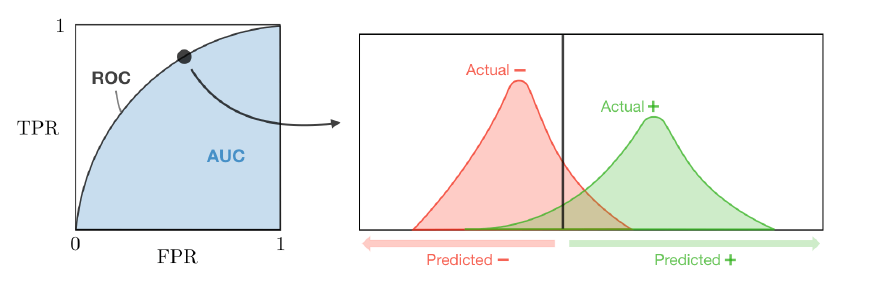
Goodness of Fit for Classification

calibration: Bin predicted probabilities $\hat{y}$ into bins $\left\{g_k\right\}$, and within each compute ${\overline{\hat{Y}}}_{g_k}$ (average predicted probability) and ${\overline{Y}}_{g_k}$. Plot the two average against each other. In a well calibrated model, the binned averages trace the identity line.

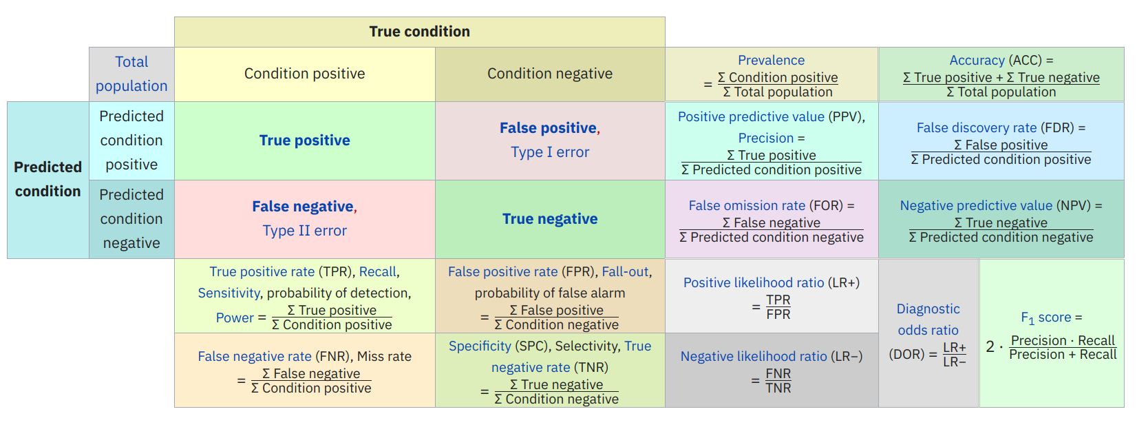
discrimination: Discrimination is a measure of whether $Y=1$ observations have high $\hat{Y}$, and correspondingly $Y=0$ values have low $\hat{Y}$. Many measures; listed below Observed $Y=1$ $Y=0$

---

Predicted positive ($\hat{Y}>c$) True Positive (TP) False Positive (FP) Predicted negative ($\hat{Y}<c$) False Negative (FN) True Negative (TN) Total Positive(P) Total Negative(N) Accuracy = $(TP+TN)/(P+N)$ - Overall performance

Precision = $TP/(TP+FP)$ - How accurate positive predictions are

Sensitivity = Recall = True positive Rate = $TP/P$ - Coverage of actual positive sample

Specificity = True Negative Rate = $TN/N$ - Coverage of actual negative sample

Brier Score =

$$\frac{1}{N}\sum _i{\left({\hat{Y}}_i-Y_i\right)}^2=\stackrel{\text{Calibration}}{\overbrace{\frac{1}{N}\sum _k^K{\left({\hat{Y}}_k-{\bar{Y}}_k\right)}^2}}+\stackrel{\text{Refinement}}{\overbrace{\frac{1}{N}\sum _k^K{n}_k\left({\bar{Y}}_k\left(1-{\bar{Y}}_k\right)\right)}}$$

F1 Score = $\frac{2TP}{2TP+FP+FN}$ : hybrid metric for unbalanced classes

Is the plot of TPR vs FPR by varying the threshold $c$.

Suppose we have a training set ${\left\{({\mathbf{X}}_i,Y_i,D_i)\right\}}_{i=1}^N$, a test point $x$, and a tree predictor

$$\hat{\mu }(x)=T(x;{\left\{({\mathbf{X}}_i,Y_i,D_i)\right\}}_{i=1}^N)$$

Equivalently,

$$\hat{\mu }(\mathbf{x})=\sum _{i=1}^n{\alpha }_i(\mathbf{x})Y_i\text{where }{\alpha }_i(\mathbf{x})=\frac{1_{{\mathbf{x}}_i\in \mathcal{L}(\mathbf{X})}}{\left|i:{\mathbf{x}}_i\in \mathcal{L}(\mathbf{x})\right|}$$

where $\mathcal{X}$ is partitioned into leaves $\mathcal{L}(x)$, where leaves are constructed to maximise heterogeneity between nodes . Do this until all leaves have $2\times$ minimum leaf size observations. Regression trees overfit, so we need to use cross-validation + other tricks.

Random forests build and average many different trees $T^{\ast }$ by

Bagging / subsampling training set (Breiman)

Selecting the splitting variable at each step from $m$ out of $p$ randomly drawn features (Amit and Geman)

$$\hat{\tau }(x)\frac{1}{B}\sum _{b=1}^B{T}_b^{\ast }(x;{\left\{({\mathbf{X}}_i,Y_i,D_i)\right\}}_{i=1}^N)$$

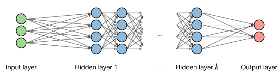
Generalised nonparametric regression with many ‘layers’, with components outline in the referenced figure. For the $i^{th}$ layer of the network and $j^{th}$ hidden layer of the unit, we have

$$z_j^{[i]}={\mathbf{w}}_j^{[i]T}\mathbf{x}+b_j^{[i]}$$

where $w,b,z$ are the weight (coefficient), bias (intercept) and output respectively.

Activation functions are used at the end of a hidden layer to introduce non-linearities into the model. Common ones are

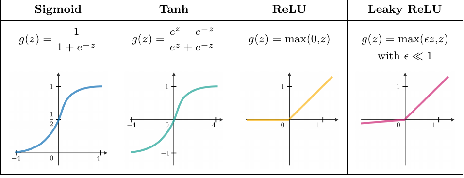
Networks frequently use the cross-entropy loss function.

Learning rate is denoted by $\eta$, which is the pace at which the weights get updated. This can be fixed or adaptively changed using ADAM.

Back-propagation is a method to update the weights in the neural net by taking into account the actual output and desired output. The derivative with respect to weight $\mathbf{w}$ is computed using the chain rule and is of the following form

$$\frac{\partial L(z,y)}{\partial w}=\frac{\partial L(z,y)}{\partial a}\frac{\partial a}{\partial z}\frac{\partial z}{\partial w}$$

So the weight is updated

$$w\leftarrow w-\eta \frac{\partial L(z,y)}{\partial w}$$

1. Take a batch of training data.
2. Perform forward propagation to compute corresponding loss.
3. Perform back propagation to compute gradients.
4. Use the gradients to update the weights over the network.

Unsupervised Learning

There is no distinction between a label/outcome $y_i$ and predictor ${\mathbf{X}}_i$ in a wide variety of problems. The goal of unsupervised methods is to characterise the joint distribution of the data $\mathbf{X}$ using latent factors, clusters, etc.

Original data $x_i$ in ${\mathbb{R}}^k$. We approximate orthogonal unit vectors $w_l\in {\mathbb{R}}^k$ and associated scores ($L\le k$ weights $z_{il}$) to minimise reconstruction error

$$J(\mathbf{X},\mathbf{\theta })=\frac{1}{n}\sum _{i=1}^n{\Vert {\mathbf{x}}_i-{\hat{\mathbf{x}}}_i\Vert }^2=\frac{1}{n}\sum _{i=1}^n{\Vert {\mathbf{x}}_i-\sum _{l=1}^L{z}_{il}{\mathbf{w}}_l\Vert }^2$$

where ${\hat{\mathbf{x}}}_i=\mathbf{W}{\mathbf{z}}_{\mathbf{i}}$ subject to the constraint that the smoother matrix $\mathbf{W}$ is orthonormal. Equivalently, the objective function can be written as

$J(\mathbf{W},\mathbf{Z})={\Vert \mathbf{X}-\mathbf{W}{\mathbf{Z}}^T\Vert }_F$ where $\mathbf{Z}$ is $N\times L$ with $z_i$ in its rows.

The optimal solution sets each ${\mathbf{w}}_l$ to be the l-th eigenvector of the empirical covariance matrix. Equivalently, $\hat{\mathbf{W}}={\mathbf{V}}_L$, which contains the $L$ eigenvectors with the largest eigenvalues of empirical covariance matrix $\hat{\mathbf{\Sigma }}=\frac{1}{n}{\sum }_{i=1}^n{\mathbf{x}}_i{\mathbf{x}}_i^{\prime }$. If we rank singular values of the data matrix $\mathbf{X}$, we can construct a rank $L$ approximation, the truncated SVD

$$\mathbf{X}\approx {\mathbf{U}}_{:,1:L}{\mathbf{S}}_{1:L,1:L}{\mathbf{V}}_{:,1:L}^{\prime }$$

This is identical to the optimal reconstruction $\hat{X}=\mathbf{Z}{\hat{\mathbf{W}}}^{\prime }$.

$$\sum _{j=L+1}^J{\lambda }_l=\text{error}(L)$$

The error is the sum of remaining eigenvalues of the covariance matrix. Total variance explained = (sum of included eigenvalues)/(sum of all eigenvalues)

Related notes

• index
• probability-and-mathstats
• linear-regression
• causal-inference