Chapter 01: Probability and Mathematical Statistics

This note is a high-fidelity Markdown migration of the Probability and Mathematical Statistics chapter from the LaTeX source.

Parent map: index

Concept map

flowchart TD
  A[Probability Space] --> B[Random Variable]
  B --> C[CDF]
  C --> D[PDF/PMF]
  C --> E[Quantile Function]
  D --> F[Expectation]
  F --> G[Variance/Covariance]
  D --> H[MGF / CGF / Characteristic Function]
  F --> I[LLN]
  G --> J[CLT]
  J --> K[Asymptotic Inference]

1. Basic Concepts and Distribution Theory

Probability

Given a measurable space $(Ω, F)$ , if $P (Ω) = 1$ , then $P$ is a probability measure and $(Ω, F, P)$ is a probability space.

sets $A \in F$ are events,
points $ω \in Ω$ are outcomes,
$P (A)$ is the probability of event $A$ .

Kolmogorov axioms

A triple $(Ω, F, P)$ is a probability space if:

Unitarity: $P (Ω) = 1$ .
Non-negativity: $P (A) \geq 0$ for all $A \in F$ .
Countable additivity: for pairwise disjoint $A_{1}, A_{2}, \dots$ , $P (i = 1 ⋃ \infty A_{i}) = i = 1 \sum \infty P (A_{i}) .$

Immediate consequences:

$A \subseteq B \Rightarrow P (A) \leq P (B)$ ,
$P (A) \leq 1$ ,
$P (A^{c}) = 1 - P (A)$ ,
$P (\emptyset) = 0$ .

Basic probability facts

For events $A, B$ :

$0 \leq P (A) \leq 1$ ,
$P (Ω) = 1$ ,
$P (\emptyset) = 0$ ,
$P (A) + P (A^{c}) = 1$ .

Random variable

A random variable is a measurable map $X : Ω \to R$ such that

{ω : X (ω) \leq x} \in F \forall x \in R .

Continuous random variable (pushforward view)

If sample space is $R$ and event space is $B (R)$ , define

P_{X} (A) = P_{ω} (ω : X (ω) \in A) = P_{ω} (X^{- 1} (A)), A \in B (R) .

DeMorgan, inclusion-exclusion, conditional probability

DeMorgan: $(A \cap B)^{c} = A^{c} \cup B^{c}$ and $(A \cup B)^{c} = A^{c} \cap B^{c}$ .
Inclusion-exclusion: $P (A \cup B) = P (A) + P (B) - P (A \cap B) .$
Conditional probability: $P (A ∣ B) = \frac{P ( A \cap B )}{P ( B )} .$

Bayes rule

P (A ∣ B) = \frac{P ( B ∣ A ) P ( A )}{P ( B )} .

Density form:

f (θ ∣ x) = \frac{f ( x ∣ θ ) f ( θ )}{\int _{θ^{'} \in Θ} f ( x ∣ θ ^{'} ) f ( θ ^{'} ) d θ ^{'}} = \frac{likelihood \times prior}{evidence} .

Statistical independence

A ⊥ B ⟺ P (A \cap B) = P (A) P (B) ⟺ P (A ∣ B) = P (A) .

2. Densities and Distributions

Distribution function (CDF)

A CDF is $F : R \to [0, 1]$ defined by

F (x) = P (X \leq x) .

Also define $F (x -) = P (X < x)$ , so

P (X = x) = F (x) - F (x -) .

Properties of CDFs:

Bounded: $lim_{x \to \infty} F (x) = 1$ , $lim_{x \to - \infty} F (x) = 0$ .
Nondecreasing: $x_{1} < x_{2} \Rightarrow F (x_{1}) \leq F (x_{2})$ .
Right-continuous: $lim_{h \to 0 +} F (x + h) = F (x)$ .
Left-limit relation: $h \to 0 + lim F (x - h) = F (x -) = F (x) - P (X = x) = P (X < x) .$

If $F^{'} (x)$ exists and

\int_{- \infty}^{\infty} F^{'} (x) d x < \infty,

then $F$ is absolutely continuous with density $f (x) = F^{'} (x)$ .

Empirical CDF for $X_{1}, \dots, X_{n}$ :

F_{n} (x) = \frac{1}{n} i = 1 \sum n 1 {X_{i} \leq x} .

Density / PMF

For continuous case,

F (x) = \int_{- \infty}^{x} f (t) d t,

so $f (x) = F^{'} (x)$ where derivative exists.

For discrete case, analogously use mass $P (X = x)$ .

Density properties:

$f (x) \geq 0$ ,
$\int_{- \infty}^{\infty} f (x) d x = 1$ .

Integration with respect to distribution function

For any measurable set $A \subset R$ ,

P (X \in A) = \int_{A} d F (x)

(Lebesgue-Stieltjes form).

If absolutely continuous:

F (x) = \int_{- \infty}^{x} f (t) d t,

and for measurable $g$ ,

\int_{- \infty}^{\infty} g (x) d F (x) = \int_{- \infty}^{\infty} g (x) f (x) d x .

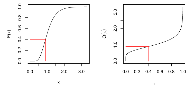
Quantile function / inverse CDF

For $τ \in (0, 1)$ ,

Q_{X} (τ) = F^{- 1} (τ) = in f {x : F (x) \geq τ} .

Check loss:

ρ_{τ} (u) = u (τ - 1 {u \leq 0}) = 1 {u > 0} τ ∣ u ∣ + 1 {u \leq 0} (1 - τ) ∣ u ∣.

For continuous $Y$ , $Q_{Y} (τ)$ minimizes expected check loss at quantile level $τ$ .

Properties of quantile functions

$Q (F (x)) \leq x$ ,
$F (Q (t)) \geq t$ ,
$Q (t) \leq x ⟺ F (x) \geq t$ ,
if strict inverse exists, $Q (t) = F^{- 1} (t)$ ,
$t_{1} < t_{2} \Rightarrow Q (t_{1}) \leq Q (t_{2})$ .

CDF and quantile function

Equivariance of quantiles under monotone transformations

If $g$ is nondecreasing and $Y$ is a random variable,

Q_{g (Y)} (τ) = g (Q_{Y} (τ)) .

Lorenz curve and Gini coefficient

For positive $Y$ with mean $μ < \infty$ and quantile function $Q_{Y}$ ,

λ (t) = μ^{- 1} \int_{0}^{t} Q_{Y} (τ) d τ .

Gini mean difference:

γ = 1 - 2 \int_{0}^{1} λ (t) d t .

2.1 Multivariate Distributions

Random vectors

A $p$ -vector random variable is $X : Ω \to R^{p}$ with components $(X_{1}, \dots, X_{p})^{'}$ .

Joint CDF:

F (x) = P (X_{1} \leq x_{1}, \dots, X_{p} \leq x_{p}) .

If continuous,

f (x) = \frac{\partial ^{p}}{\partial x _{1} \dots \partial x _{p}} F (x) .

Marginals and conditionals

For coordinate $i$ :

F_{X_{i}} (x_{i}) = F (\infty, \dots, \infty, x_{i}, \infty, \dots, \infty),

f_{X_{i}} (x_{i}) = \int_{R^{p - 1}} f (x) d x_{- i} .

Conditional density for $X_{1} ∣ X_{- 1} = x_{- 1}$ :

f_{X_{1} ∣ X_{- 1}} (x_{1} ∣ x_{- 1}) = \frac{f ( x )}{f _{X_{- 1}} ( x _{- 1} )} .

For bivariate $f_{X, Y}$ :

f_{X} (x) = \int_{- \infty}^{\infty} f_{X, Y} (x, y) d y,

f_{Y ∣ X} (y ∣ x) = \frac{f _{X, Y} ( x , y )}{f _{X} ( x )} .

Independence (distributional statements)

$X$ and $Y$ are independent if

f_{X, Y} (x, y) = f_{X} (x) f_{Y} (y) .

Useful implications under independence:

$Cov (X, Y) = 0$ ,
$ρ (X, Y) = 0$ ,
$Var (X + Y) = Var (X) + Var (Y)$ .

3. Moments

For random variable $X$ with support $[\underline{x}, \overset{x}{ˉ}]$ :

$n$ th raw moment: $μ_{n}^{'} = E [X^{n}]$ ,
$n$ th central moment: $μ_{n} = E [(X - E X)^{n}]$ .

Expectation and variance

Expectation is the Lebesgue-Stieltjes integral of $X$ with respect to $P$ .

Equivalent notation includes $E [X]$ and $\int X d P$ .

E [X] = \int_{\underline{x}}^{\overset{x}{ˉ}} x d F (x) = \int_{\underline{x}}^{\overset{x}{ˉ}} x f (x) d x (if absolutely continuous) .

Var (X) = E [(X - E X)^{2}] = E [X^{2}] - (E X)^{2} .

Variance-covariance matrix

For vectors:

Var (X) = E (X X^{'}) - E (X) E (X)^{'},

Cov (X, Y) = E [(X - E X) (Y - E Y)^{'}] .

Skewness and kurtosis

Skewness = γ = \frac{E [( X - μ ) ^{3} ]}{σ ^{3}},

Excess kurtosis = κ = \frac{E [( X - μ ) ^{4} ]}{σ ^{4}} - 3.

Linear transformations

For matrix $A$ and vector random variable $X$ with covariance $Σ$ :

Cov (A X + b) = A Σ A^{'} .

If $X \sim N (μ, Σ)$ :

A X + y \sim N (A μ + y, A Σ A^{'}) .

Also,

(X - μ)^{'} Σ^{- 1} (X - μ) \sim χ_{n}^{2}

in the standard multivariate normal setup with matching dimension.

Law of the unconscious statistician (LOTUS)

If $Y = r (X)$ ,

E [Y] = E [r (X)] = \int r (x) d F (x) = \int r (x) f (x) d x .

Linear combinations and covariance algebra

E [a X + bY] = a E [X] + b E [Y],

Var (a X) = a^{2} Var (X),

Var (a X + bY) = a^{2} Var (X) + b^{2} Var (Y) + 2 ab Cov (X, Y),

Cov (a X + c, bY + d) = ab Cov (X, Y) .

For vectors,

Var (A X + b) = A Var (X) A^{'} .

Moment generating function (MGF) and Laplace transform

For nonnegative $X$ , Laplace transform:

L_{X} (t) = E [e^{- tX}], t \geq 0.

MGF:

M_{X} (t) = E [e^{tX}] .

If MGF exists around $0$ ,

M_{X} (t) = j = 0 \sum \infty t^{j} \frac{E [ X ^{j} ]}{j !},

E [X^{n}] = M_{X}^{(n)} (0) .

Cumulant generating function (CGF)

K_{X} (t) = lo g M_{X} (t)

with expansion

K_{X} (t) = j = 1 \sum \infty \frac{κ _{j}}{j !} t^{j},

where cumulants are

κ_{j} = K_{X}^{(j)} (0) .

Characteristic function

ϕ_{X} (t) = E [e^{i tX}] = E [cos (tX)] + i E [sin (tX)], t \in R .

If MGF exists, $M_{X} (i t) = ϕ_{X} (t)$ . Characteristic functions always exist.

Order statistics

If $X_{1}, \dots, X_{n}$ are i.i.d. with CDF $F$ and PDF $f$ , then density of $k$ th order statistic $X_{(k)}$ is

f_{X_{(k)}} (x) = \frac{n !}{( k - 1 )! ( n - k )!} F (x)^{k - 1} (1 - F (x))^{n - k} f (x) .

Correlation coefficient

ρ (X, Y) = \frac{Cov ( X , Y )}{σ _{X} σ _{Y}} \in [- 1, 1] .

$ρ (X, Y) = 1$ iff $Y = a + b X$ with $b > 0$ ,
$ρ (X, Y) = - 1$ iff $Y = a - b X$ with $b > 0$ .

Entropy, KL divergence, and mutual information

For discrete random variable with PMF $p (x)$ ,

H (X) = - x \in X \sum p (x) lo g_{b} p (x) .

Properties include:

$H (X) \geq 0$ ,
change of base relation,
conditioning reduces entropy: $H (X ∣ Y) \leq H (X)$ ,
$H (X) \leq lo g ∣ X ∣$ with equality for uniform,
$H (p)$ is concave in $p$ .

Relative entropy (KL divergence):

D (p ∥ q) = x \sum p (x) lo g \frac{p ( x )}{q ( x )} .

Mutual information:

I (X; Y) = x \sum y \sum p (x, y) lo g \frac{p ( x , y )}{p ( x ) p ( y )} .

Equivalent forms:

I (X; Y) = H (X) - H (X ∣ Y) = H (Y) - H (Y ∣ X) = H (X) + H (Y) - H (X, Y) .

Copulas and Fréchet bounds

For random variables $(X, Y)$ with marginals $F, H$ and joint CDF $G$ ,

C (u, v) = G (F^{- 1} (u), H^{- 1} (v)), C : [0, 1]^{2} \to [0, 1] .

Fréchet bounds:

max {F (x) + H (y) - 1, 0} \leq G (x, y) \leq min {F (x), H (y)} .

Special cases:

upper bound: comonotonic dependence,
lower bound: countermonotonic dependence,
independence: $C (u, v) = uv$ .

4. Transformations of Random Variables

4.1 Useful inequalities

The central question is to bound tail probabilities such as

P (∣ X - E X ∣ \geq t), t \geq 0.

Cauchy-Schwarz

For random variables with finite second moments,

E [∣ X Y ∣] \leq E [X^{2}] E [Y^{2}] .

Hence

Cov (X, Y)^{2} \leq Var (X) Var (Y) .

Jensen

If $g$ is concave and expectations exist,

E [g (Y)] \leq g (E [Y]) .

If $f$ is convex,

E [f (X)] \geq f (E [X]) .

Markov

For nonnegative $ψ$ and $t > 0$ ,

P (ψ (X) \geq t) \leq \frac{E [ ψ ( X )]}{t} .

Special case:

P (∣ X ∣ > ϵ) \leq \frac{E [ ∣ X ∣ ^{r} ]}{ϵ ^{r}}, r \geq 1.

Chebyshev

If $E [X] = μ$ and $Var (X) = σ^{2} < \infty$ ,

P (∣ X - μ ∣ > ϵ) \leq \frac{σ ^{2}}{ϵ ^{2}} .

Kolmogorov inequality (as stated in source notes)

For independent mean-zero variables with finite second moments,

P (1 \leq j \leq n max ∣ X_{j} ∣ \geq ϵ) \leq \frac{\sum _{j} E [ X _{j}^{2} ]}{ϵ ^{2}} .

Chernoff-type bound identity

For any random variable $Z$ and $t \geq 0$ ,

P (Z \geq E Z + t) \leq λ \geq 0 in f E [e^{λ (Z - E Z)}] e^{- λ t} = λ \geq 0 in f M_{Z - E Z} (λ) e^{- λ t} .

Hölder

For $p, q > 1$ with $1/ p + 1/ q = 1$ ,

E [∣ g_{1} (X) g_{2} (X) ∣] \leq E [∣ g_{1} (X) ∣^{p}]^{1/ p} E [∣ g_{2} (X) ∣^{q}]^{1/ q} .

Hoeffding lemma form

If $a \leq X \leq b$ , then for all $s \in R$ ,

lo g E [e^{s X}] \leq s E [X] + \frac{s ^{2} ( b - a ) ^{2}}{8} .

5. Transformations and Conditional Distributions

Let $Y = g (X)$ .

CDF method for transformations

F_{Y} (y) = P (Y \leq y) = P (g (X) \leq y) = F_{X} (g^{- 1} (y))

for monotone invertible $g$ .

Change of variables for density

Scalar case:

f_{Y} (y) = f_{X} (g^{- 1} (y)) \frac{d}{d y} g^{- 1} (y) .

Multivariate case:

f_{Y} (y) = f_{X} (g^{- 1} (y)) det J_{g^{- 1}} (y) = f_{X} (g^{- 1} (y)) det J_{g} (g^{- 1} (y))^{- 1} .

Example: $Y = X^{2}$ when $f_{X} (x) = 3 x^{2}$

If $g^{- 1} (y) = y^{1/2}$ ,

\frac{d}{d y} g^{- 1} (y) = \frac{1}{2} y^{- 1/2},

f_{Y} (y) = f_{X} (y^{1/2}) \frac{1}{2} y^{- 1/2} = 3 (y^{1/2})^{2} \cdot \frac{1}{2} y^{- 1/2} = \frac{3}{2} y^{1/2} .

Conditional expectation

For jointly continuous $(X, Y)$ ,

E [Y ∣ X = x] = \int y f_{Y ∣ X} (y ∣ x) d y .

For function $h$ ,

E [h (X, Y) ∣ X = x] = \int h (x, y) f_{Y ∣ X} (y ∣ x) d y .

Conditional variance

Var (Y ∣ X) = E [(Y - E [Y ∣ X])^{2} ∣ X] = E [Y^{2} ∣ X] - E [Y ∣ X]^{2} .

Law of iterated expectations

E [Y] = E [E [Y ∣ X]] .

Law of total variance

Var (Y) = E [Var (Y ∣ X)] + Var (E [Y ∣ X]) .

5.1 Distribution facts and links

Normal facts

If $X \sim N (μ_{X}, σ_{X}^{2})$ and $Y \sim N (μ_{Y}, σ_{Y}^{2})$ :

$W = a X + b \sim N (a μ_{X} + b, a^{2} σ_{X}^{2})$ ,
if $X ⊥ Y$ , then $X + Y \sim N (μ_{X} + μ_{Y}, σ_{X}^{2} + σ_{Y}^{2})$ .

Multivariate normal

For $X \sim N_{p} (μ, Σ)$ ,

ϕ_{Σ} (x) = \frac{1}{( 2 π ) ^{p /2} ∣Σ ∣ ^{1/2}} exp (- \frac{1}{2} (x - μ)^{'} Σ^{- 1} (x - μ)) .

Linear image:

A X + b \sim N_{q} (A μ + b, A Σ A^{'}) .

Common links

Student- $t$ from normal over square-root chi-square ratio,
$F$ from ratio of scaled chi-square variables,
Bernoulli as Binomial $(1, p)$ ,
Uniform $(0, 1)$ as Beta $(1, 1)$ ,
Exponential as Gamma $(1, λ)$ ,
$χ_{n}^{2}$ as Gamma $(n /2, 1/2)$ ,
Geometric as NegBin $(1, p)$ .

Misc facts

Exponential is memoryless: $P (X > s + t ∣ X > s) = P (X > t) .$
Poisson inter-arrival times are exponential.
If $X \sim Γ (a, λ)$ , then $X$ is wait time to $a$ arrivals in a Poisson process of rate $λ$ .

Exchangeability

$X_{1}, \dots, X_{n}$ are exchangeable if any permutation has the same joint distribution.

Martingales

A sequence ${X_{n}}$ with $E ∣ X_{n} ∣ < \infty$ is a martingale if

E [X_{n + 1} ∣ X_{1}, \dots, X_{n}] = X_{n} .

6. Statistical Decision Theory

A statistical decision problem is a game between nature and a decision maker.

Nature chooses $θ \in Θ$ and generates data from $P_{θ}$ .
DM observes data and chooses action $a \in A$ .
Utility/loss depends on $(a, θ)$ .

Statistical problem tuple

(Θ, A, u (\cdot), {P_{θ}}) .

A decision rule is $d : X \to A$ .

Example: estimation

action space $A = Θ$ ,
decision rule is estimator,
common loss: quadratic loss $(a - θ)^{2}$ .

Example: testing

Partition $Θ$ into null $Θ_{0}$ and alternative $Θ_{1}$ .

action space ${a_{0}, a_{1}}$ ,
decision rule is test,
common loss: zero-one misclassification loss.

Example: interval inference

Actions are confidence sets $a \subseteq R$ .

Risk and admissibility

Risk of $d$ :

R (θ; d) = E_{P_{θ}} [L (d (X), θ)] .

$d$ is dominated by $d^{'}$ if $R (θ; d^{'}) \leq R (θ; d)$ for all $θ$ . Undominated rules are admissible.

James-Stein shrinkage example

If $Y_{i} \sim N (μ_{i}, 1)$ , estimate vector $μ$ under squared loss

L (\overset{μ}{^}, μ) = i \sum (\overset{μ}{^}_{i} - μ_{i})^{2} .

MLE is $\overset{μ}{^} = Y$ , but for $n \geq 3$ , shrinkage estimator

\overset{μ}{^}_{i} = (1 - \frac{n - 2}{\sum _{i} Y _{i}^{2}}) Y_{i}

has lower risk than the coordinatewise MLE.

Bayes risk and Bayes rule

Given prior $π$ on $Θ$ :

r (π, d) = \int_{Θ} R (θ, d) d π (θ) .

A Bayes rule minimizes $r (π, d)$ over admissible $d$ .

Minimax

$d_{0}$ is minimax if

θ \in Θ sup R (θ, d_{0}) = d \in D in f θ \in Θ sup R (θ, d) .

7. Estimation

Sample statistic

For i.i.d. $X_{1}, \dots, X_{n}$ , a sample statistic is

T_{n} = h_{n} (X_{1}, \dots, X_{n}) .

Unbiasedness

$\hat{θ}$ is unbiased if

E [\hat{θ}] = θ .

Consistency

$\hat{θ}$ is consistent if

\hat{θ} p θ .

Asymptotic normality

n (\hat{θ} - θ) d N (0, V_{\hat{θ}}) .

Sampling variance

For estimator $\hat{θ}$ , sampling variance is $Var (\hat{θ})$ .

Mean squared error (MSE)

MSE (\hat{θ}) = E [(\hat{θ} - θ)^{2}] = (E [\hat{θ}] - θ)^{2} + Var (\hat{θ}) .

Also,

ar g c \in R min E [(X - c)^{2}] = E [X] .

Mean and variance estimators

$\overset{ˉ}{X} = \frac{1}{n} \sum_{i} X_{i}$ is unbiased for $E [X]$ ,
$S_{X}^{2} = \frac{1}{n - 1} \sum_{i} (X_{i} - \overset{ˉ}{X})^{2}$ is unbiased for $Var (X)$ .

If $X_{i} \sim N (μ, σ^{2})$ :

$\overset{ˉ}{X} \sim N (μ, σ^{2} / n)$ ,
$\frac{n - 1}{σ ^{2}} S_{X}^{2} \sim χ_{n - 1}^{2}$ ,
$\overset{ˉ}{X}$ and $S_{X}^{2}$ are independent,
$\frac{X ˉ - μ}{S _{X}^{2} / n} \sim t_{n - 1} .$

8. Hypothesis Testing

Test statistic and test

A test statistic is a sample function $S_{n} = T (X_{1}, \dots, X_{n})$ . A test is a map from statistic space to ${0, 1}$ (reject / do not reject).

Standard normal-style statistic:

s = \frac{θ ^ - θ _{0}}{ω},

with rejection in two-sided test when $s > z_{1 - α /2}$ .

Null and alternative

$H_{0} : θ \in Θ_{0}$ is maintained unless contradicted,
$H_{1} : θ \in Θ_{1}$ is alternative.

Decision rule partitions statistic support into acceptance and rejection regions.

Type I/II, power

Decision	Null true	Null false
Reject $H_{0}$	Type I error $α$	Power
Do not reject $H_{0}$	$1 - α$	Type II error $1 - Power$

Power function:

π (θ) = P_{θ} (S \in R) .

Size of test:

θ \in Θ_{0} sup P_{θ} (S \in R) .

Two-sided normal-approximation confidence interval

C I_{1 - α} (θ) = [\hat{θ} - z_{1 - α /2} V [\hat{θ}], \hat{θ} + z_{1 - α /2} V [\hat{θ}]] .

P-values

two-sided: $p = 2 {1 - Φ (∣ s ∣)}$ ,
one-sided: $p = 1 - Φ (s)$ or $Φ (s)$ depending on alternative direction.

9. Convergence Concepts

Asymptotics studies how estimators behave as $n \to \infty$ , often targeting asymptotic normality of scaled errors.

Modes of convergence

For sequence $X_{n}$ :

in probability: $X_{n} p X$ ,
in mean square: $X_{n} L_{2} X$ if $E [(X_{n} - X)^{2}] \to 0$ ,
in distribution: $X_{n} d X$ .

Standard implications:

$X_{n} L_{2} X \Rightarrow X_{n} p X$ ,
$X_{n} p X \Rightarrow X_{n} d X$ ,
$X_{n} a . s . X \Rightarrow X_{n} p X$ ,
if limit is constant $c$ , $X_{n} d c \Rightarrow X_{n} p c$ .

9.1 Laws of Large Numbers

Basic statement:

\frac{1}{n} i = 1 \sum n (Z_{i} - E Z_{i}) p 0.

Chebyshev LLN

If i.i.d. with finite mean and variance,

\frac{1}{n} i = 1 \sum n X_{i} p E [X_{1}] .

Strong LLN

Under standard finite-variance conditions,

\overset{ˉ}{X} a . s . μ .

Glivenko-Cantelli

For i.i.d. sample from CDF $F$ ,

F_{n} (x) = \frac{1}{n} i = 1 \sum n 1 {X_{i} \leq x}

obeys

x \in R sup ∣ F_{n} (x) - F (x) ∣ a . s . 0.

This gives consistency of the empirical CDF and empirical quantiles.

9.2 Central Limit Theorem

For i.i.d. with mean $μ$ and variance $σ^{2}$ ,

n (\overset{ˉ}{X}_{n} - μ) d N (0, σ^{2}),

or equivalently

\frac{X ˉ _{n} - μ}{σ / n} d N (0, 1) .

9.3 Tools for transformations

Continuous mapping theorem

If $X_{n} d X$ and $h$ continuous, then $h (X_{n}) d h (X)$ .
If $X_{n} p X$ and $h$ continuous, then $h (X_{n}) p h (X)$ .

Slutsky

If $X_{n} d X$ and $Y_{n} p c$ ,

$X_{n} + Y_{n} d X + c$ ,
$X_{n} Y_{n} d X c$ ,
$X_{n} / Y_{n} d X / c$ if $c \neq = 0$ .

Delta method

n (\hat{θ}_{n} - θ) d N (0, Σ)

and $g$ is continuously differentiable at $θ$ , then

n (g (\hat{θ}_{n}) - g (θ)) d N (0, \nabla g (θ) Σ\nabla g (θ)^{'}) .

Scalar form:

n (g (t_{n}) - g (θ)) d N (0, g^{'} (θ)^{2} σ^{2}) .

9.4 Orders of magnitude

For deterministic functions $u, v$ as argument approaches $L$ :

$u = O (v)$ if $∣ u / v ∣$ bounded,
$u = o (v)$ if $u / v \to 0$ ,
$u \sim v$ if $u / v \to 1$ .

Constant order means $f (n) = O (1)$ .

9.5 Stochastic orders

For sequences:

$Z_{n} = O_{p} (a_{n})$ means $Z_{n} / a_{n}$ is stochastically bounded,
$Z_{n} = o_{p} (a_{n})$ means $Z_{n} / a_{n} p 0$ .

Common identities:

$o_{p} (1) + o_{p} (1) = o_{p} (1)$ ,
$O_{p} (1) + O_{p} (1) = O_{p} (1)$ ,
$o_{p} (1) \cdot O_{p} (1) = o_{p} (1)$ ,
$O_{p} (1) \cdot O_{p} (1) = O_{p} (1)$ .

Example consistency decomposition:

\hat{β} = β + O_{p} (1) o_{p} (1) = β + o_{p} (1) p β .

10. Parametric Models

Parametric model

For outcome $Y$ and covariates $X$ , a parametric model is

P = {P (y, x; θ) : θ \in Θ}

with finite-dimensional parameter $θ$ .

Model is true if there exists $θ \in Θ$ such that

f_{Y ∣ X} (y ∣ x) = g (y, x; θ) .

Identifiability means distinct parameters imply distinct distributions:

θ_{1} \neq = θ_{2} \Rightarrow P (\cdot; θ_{1}) \neq = P (\cdot; θ_{2}) .

Regression model view

Independent (not necessarily identically distributed) $Y_{j}$ with parameter $λ_{j}$ , and known covariates $x_{j}$ satisfy

λ_{j} = h (x_{j}, θ) .

$h$ is known; $θ$ is unknown.

Classical linear model example

g (y, x; (β, σ)) = ϕ (y; x^{'} β, σ^{2}),

with parameter space

Θ = {(β, σ) \in R^{k + 1} : σ \geq 0} .

Binary choice example

For $y \in {0, 1}$ ,

g (y, x; β) = {1 - h (x^{'} β), h (x^{'} β), y = 0, y = 1,

with known link $h$ (logit/probit).

Fisher-Neyman factorization theorem

Statistic $ϕ (x)$ is sufficient for $θ$ iff

p (x ∣ θ) = h (x) g_{θ} (ϕ (x)) .

Equivalent Bayesian statement: posterior depends on $x$ only through $ϕ (x)$ .

11. Robustness

Write estimators as functionals of empirical CDF:

\hat{θ}_{n} = θ_{n} (F_{n}), F_{n} (y) = \frac{1}{n} i \sum 1 {y_{i} \leq y} .

Examples:

mean: $θ_{n} = \int y d F_{n} (y)$ ,
median: $θ_{n} = F_{n}^{- 1} (1/2)$ ,
trimmed mean: $θ_{n} = \frac{1}{1 - 2 α} \int_{α}^{1 - α} F_{n}^{- 1} (u) d u .$

Let $L_{F} (θ_{n})$ denote distribution of estimator under data law $F$ .

Prokhorov distance

For probability measures $F, G$ on metric space,

π (F, G) = in f {ϵ : F [A] \leq G [A^{ϵ}] + ϵ \forall A \in B} .

Hampel robustness

Estimator sequence ${θ_{n}}$ is robust at $F$ if

\forall ϵ > 0, \exists δ > 0 : π (F, G) < δ \Rightarrow π (L_{F} (θ_{n}), L_{G} (θ_{n})) < ϵ \forall n .

Influence function

For contamination model $F_{ϵ} = (1 - ϵ) F + ϵ δ_{x}$ ,

IF_{θ, F} (x) = ϵ \to 0 lim \frac{θ ( F _{ϵ} ) - θ ( F )}{ϵ} .

Examples from notes:

mean: $IF (x) = x - μ (F)$ ,
variance: $IF (x) = (x - μ)^{2} - σ^{2}$ .

Both are unbounded as $∣ x ∣ \to \infty$ , highlighting non-robustness to outliers.

12. Identification

A data-generating process (DGP) fully specifies the stochastic process generating observables.

A model $M$ is a family of admissible DGPs and can be:

parametric,
nonparametric,
semiparametric.

Semiparametric OLS example

y_{i} = x_{i}^{'} β + ϵ_{i},

E [ϵ_{i} ∣ x_{i}] = 0,

with finite-dimensional $β$ and otherwise unrestricted joint law.

Index-model semiparametric example

y_{i} = g (x_{i}^{'} β) + ϵ_{i},

E [ϵ_{i} ∣ x_{i}] = 0,

where $g$ and error distribution are nuisance objects.

Generic nonparametric model

Y_{i} = g (x_{i}, ϵ_{i}), x_{i} ⊥ ϵ_{i},

with unrestricted marginals and target functionals such as $E_{ϵ} [g (x_{i}, ϵ_{i})]$ .

Structural representation

Many models can be represented as

Y_{i} = g (U_{i}), U_{i} \sim ii d F_{U},

with structure

θ = (g, F_{U}) .

Identified set

If $F_{Y}$ is observed distribution and $F_{θ}$ is implied by structure $θ$ , then

Ω (F_{Y}, Θ) = {θ \in Θ : F_{θ} (\cdot) = F_{Y} (\cdot)} .

point identified: $Ω$ is singleton,
partial identification: $Ω$ has multiple elements.

Observational equivalence

$θ^{'}$ and $θ^{''}$ are observationally equivalent if

F_{θ^{'}} (y) = F_{θ^{''}} (y) \forall y .

Ceteris paribus effect in structural model

For $Y_{i} = f (X_{i}, U_{i}; ϕ)$ ,

Δ_{i} (x^{''}, x^{'}) = f (x^{''}, U_{i}; ϕ) - f (x^{'}, U_{i}; ϕ) .

If $X_{i} ⊥ U_{i}$ and structure is identified, distribution of causal effects can be identified.

Statistical functionals and estimands

If model-indexed laws are

P_{Θ} = {P_{θ} (Y, {Y^{d}}_{d \in D}, X) : θ \in Θ},

then a functional is a map

ψ (\cdot) : P_{Θ} \to R .

In causal inference, such functionals are estimands.

Lalgorithms

Explorer