Chapter 02: Linear Regression

This note is a high-fidelity Markdown migration of the Linear Regression chapter from the LaTeX source.

Parent map: index Prerequisites: probability-and-mathstats

Concept map

flowchart TD
  A[Simple Linear Regression] --> B[OLS Estimator]
  B --> C[Finite-sample Properties]
  C --> D[Gauss-Markov BLUE]
  C --> E[Prediction / Intervals]
  B --> F[Projection Geometry]
  F --> G[FWL / Partitioned Regression]
  C --> H[Robust SEs]
  H --> I[Hypothesis Testing]
  I --> J[Multiple Testing]
  B --> K[Quantile Regression]
  B --> L[Measurement Error]
  B --> M[Bootstrap / Delta Method]
  B --> N[GMM]
  N --> O[Empirical Likelihood]
  N --> P[M-estimation]

1. Simple Linear Regression

Assume

$$Y_i={\beta }_0+{\beta }_1{X}_i+{\epsilon }_i,$$

with

$$\mathbb{E}[{\epsilon }_i\mid X_i]=0,\mathrm{Var}({\epsilon }_i\mid X_i)={\sigma }^2.$$

1.1 OLS in summation form

Population best linear predictor coefficients:

$${\beta }_1=\frac{\mathrm{Cov}(X,Y)}{\mathrm{Var}(X)},{\beta }_0=\mathbb{E}[Y]-{\beta }_1\mathbb{E}[X].$$

Sample analogues:

$${\hat{\beta }}_1=\frac{{\sum }_i(X_i-\bar{X})(Y_i-\bar{Y})}{{\sum }_i(X_i-\bar{X}{)}^2}=\frac{\overline{XY}-\bar{X}\bar{Y}}{\overline{X^2}-{\bar{X}}^2},$$ $${\hat{\beta }}_0=\bar{Y}-{\hat{\beta }}_1\bar{X}.$$

Residual variance estimate in simple regression:

$${\hat{\sigma }}^2=\frac{{\sum }_i{\hat{\epsilon }}_i^2}{n-2}.$$

Variance decomposition from the fitted line $\hat{Y}={\hat{\beta }}_0+{\hat{\beta }}_{1}X$ and residual $U=Y-\hat{Y}$:

$$\mathrm{Var}(\hat{Y})={\rho }_{XY}^2{\sigma }_Y^2,\mathrm{Var}(U)=(1-{\rho }_{XY}^2){\sigma }_Y^2.$$

1.2 Properties of least-squares estimators

Let $\hat{\beta }=({\hat{\beta }}_0,{\hat{\beta }}_1{)}^{\prime }$. Conditionally on regressors:

$$\mathbb{E}[\hat{\beta }\mid X]=\left(\begin{array}{c}{\beta }_0\\ {\beta }_1\end{array}\right),$$ $$\mathrm{Var}(\hat{\beta }\mid X)=\frac{{\sigma }^2}{n{s}_X^2}\left(\begin{array}{cc}\frac{1}{n}{\sum }_i{X}_i^2& -\bar{X}\\ -\bar{X}& 1\end{array}\right),$$

where

$$s_X^2=\frac{1}{n}\sum _i(X_i-\bar{X}{)}^2,S_{xx}=\sum _i(X_i-\bar{X}{)}^2.$$

Component formulas:

$$\mathrm{Var}({\hat{\beta }}_0)={\sigma }^2\left(\frac{1}{n}+\frac{{\bar{X}}^2}{S_{xx}}\right),$$ $$\mathrm{Var}({\hat{\beta }}_1)=\frac{{\sigma }^2}{S_{xx}}=\frac{{\sigma }^2}{n\mathrm{Var}(X)}.$$

Heteroskedastic scalar-regression asymptotic expression:

$$\mathrm{Var}({\hat{\beta }}_1)\approx \frac{\mathrm{Var}((X_i-\bar{X})u_i)}{n\mathrm{Var}(X_i-\bar{X}{)}^2}.$$

With multiple regressors, a useful form is

$$\mathrm{Var}({\hat{\beta }}_j)=\frac{{\sigma }^2}{{\mathrm{TSS}}_j(1-R_j^2)},$$

where $R_j^2$ is from regressing regressor $X_j$ on the other regressors and an intercept. This denominator gives the variance-inflation interpretation.

1.3 Prediction

For new covariate value $x_0$:

$${\hat{y}}_0={\hat{\beta }}_0+{\hat{\beta }}_1{x}_0.$$

Prediction-mean variance:

$$\mathrm{Var}({\hat{y}}_0)=\mathrm{Var}({\hat{\beta }}_0)+x_0^2\mathrm{Var}({\hat{\beta }}_1)+2x_0\mathrm{Cov}({\hat{\beta }}_0,{\hat{\beta }}_1)={\sigma }^2\left(\frac{1}{n}+\frac{(x_0-\bar{X}{)}^2}{S_{xx}}\right).$$

Forecast error $e_f=y_0-{\hat{y}}_0$ has

$$\mathrm{Var}(e_f)={\sigma }^2+\mathrm{Var}({\hat{y}}_0).$$

Estimated prediction variance:

$${\hat{\xi }}^2={\hat{\sigma }}^2\left(1+\frac{1}{n}+\frac{(x_0-\bar{X}{)}^2}{S_{xx}}\right).$$

1.4 Simple regression in matrix form

With $X=[1,x]$,

$$X^{\prime }X=\left(\begin{array}{cc}{1}^{\prime }1& 1^{\prime }x\\ x^{\prime }1& x^{\prime }x\end{array}\right).$$

Using block inversion, one can recover the standard simple-regression closed forms and show

$$\hat{\beta }=(X^{\prime }X{)}^{-1}{X}^{\prime }y.$$

2. Classical Linear Model

2.1 Assumptions

A common stack of assumptions:

1. Linearity: $Y=X\beta +\epsilon$.
2. Exogeneity (strict/conditional): $\mathbb{E}[\epsilon \mid X]=0$.
3. Spherical errors: $\mathrm{Var}(\epsilon \mid X)={\sigma }^2{I}_n$.
4. Full column rank: $\mathrm{rank}(X)=k$.
5. Normal errors (for exact finite-sample normality): $\epsilon \mid X\sim \mathcal{N}(0,{\sigma }^2{I}_n)$.
6. I.I.D. sampling of $(Y_i,X_i)$ when using random-design asymptotics.

Notes:

• Assumptions 1-4 give unbiasedness and Gauss-Markov efficiency statements.
• Replacing homoskedasticity with $\mathrm{Var}(\epsilon \mid X)=\Omega$ yields $$\hat{\beta }\mid X\sim \mathcal{N}\left(\beta ,(X^{\prime }X{)}^{-1}{X}^{\prime }\Omega X(X^{\prime }X{)}^{-1}\right)$$ under normality.

2.2 Optimization derivation of OLS

OLS solves

$$\underset{\beta \in {\mathbb{R}}^k}{\min }(y-X\beta {)}^{\prime }(y-X\beta ).$$

FOC:

$$-2X^{\prime }(y-X\beta )=0\Rightarrow X^{\prime }X\hat{\beta }=X^{\prime }y\Rightarrow \hat{\beta }=(X^{\prime }X{)}^{-1}{X}^{\prime }y.$$

With fixed regressors and homoskedasticity:

$$\mathrm{Var}(\hat{\beta })={\sigma }^2(X^{\prime }X{)}^{-1},{\hat{\sigma }}^2=\frac{e^{\prime }e}{n-k},e=y-X\hat{\beta }.$$

3. Finite and Large Sample Properties of $\hat{\beta }$ and ${\hat{\sigma }}^2$

3.1 Finite-sample unbiasedness (conditional on $X$)

Under linear model + exogeneity,

$$\mathbb{E}[\hat{\beta }\mid X]=\mathbb{E}\left[(X^{\prime }X{)}^{-1}{X}^{\prime }(X\beta +\epsilon )\mid X\right]=\beta +(X^{\prime }X{)}^{-1}{X}^{\prime }\mathbb{E}[\epsilon \mid X]=\beta .$$

A common caveat in the source notes: if you try to manipulate unconditional expectations through random matrix inverses directly, naive ratio-of-expectations shortcuts fail.

3.2 Finite-sample variance

$$\mathrm{Var}(\hat{\beta }\mid X)=(X^{\prime }X{)}^{-1}{X}^{\prime }\mathbb{E}[\epsilon {\epsilon }^{\prime }\mid X]X(X^{\prime }X{)}^{-1}={\sigma }^2(X^{\prime }X{)}^{-1}$$

under homoskedasticity.

With normality:

$$\hat{\beta }\mid X\sim \mathcal{N}(\beta ,{\sigma }^2(X^{\prime }X{)}^{-1}).$$

3.3 Gauss-Markov (BLUE)

Within linear unbiased estimators, OLS has minimum variance: for any linear unbiased $b$,

$$a^{\prime }\left(\mathrm{Var}(\hat{\beta }\mid X)-\mathrm{Var}(b\mid X)\right)a\le 0$$

in PSD ordering (equivalently $\mathrm{Var}(b)-\mathrm{Var}(\hat{\beta })$ is PSD).

3.4 Large-sample conditions and consistency

Typical conditions in the notes:

• finite positive-definite $\mathbb{E}[X_i{X}_i^{\prime }]$,
• fourth moments of regressors and errors finite,
• positive-definite $\mathbb{E}[{\epsilon }_i^2{X}_i{X}_i^{\prime }]$.

Consistency decomposition:

$$\hat{\beta }-\beta ={\left(\frac{1}{n}\sum _i{X}_i{X}_i^{\prime }\right)}^{-1}\left(\frac{1}{n}\sum _i{X}_i{\epsilon }_i\right)\stackrel{p}{\to }0.$$

3.5 Asymptotic normality and sandwich variance

$$\sqrt{n}(\hat{\beta }-\beta )\stackrel{d}{\to }\mathcal{N}(0,A^{-1}B{A}^{-1}),$$

with

$$A=\mathbb{E}[X_i{X}_i^{\prime }],B=\mathbb{E}[{\epsilon }_i^2{X}_i{X}_i^{\prime }].$$

Sample robust (Huber-White) form:

$$\widehat{\mathrm{Var}}(\hat{\beta })=(X^{\prime }X{)}^{-1}{X}^{\prime }\hat{\Omega }X(X^{\prime }X{)}^{-1},\hat{\Omega }=\mathrm{diag}({\hat{e}}_1^2,\dots ,{\hat{e}}_n^2).$$

In scalar simple regression this reduces to

$$\mathrm{Var}(\hat{\beta })\approx \frac{\mathbb{E}[{\epsilon }^2(X-\mathbb{E}X{)}^2]}{n\mathrm{Var}(X{)}^2}.$$

3.6 Unbiasedness of ${\hat{\sigma }}^2$

Using $e=M_X\epsilon$ and $M_X=I-P_X$,

$$\mathbb{E}[e^{\prime }e\mid X]=\mathbb{E}[{\epsilon }^{\prime }{M}_X\epsilon \mid X]={\sigma }^2\mathrm{tr}(M_X)={\sigma }^2(n-k).$$

Hence ${\hat{\sigma }}^2=e^{\prime }e/(n-k)$ is unbiased conditionally on $X$.

3.7 Polynomial approximation and sieve intuition

Wierstrass theorem in this context supports approximating continuous conditional mean functions on compact support by high-order polynomials.

A polynomial sieve estimator of $m(x)=\mathbb{E}[Y\mid X=x]$ takes

$$\hat{m}(x)=\sum _{j=0}^{J_n}{\hat{\beta }}_j{x}^j,$$

where $J_n\to \infty$ but $J_n/n\to 0$ for consistency.

4. Geometry of OLS

Define

$$P_X=X(X^{\prime }X{)}^{-1}{X}^{\prime }\text{(hat matrix)},$$ $$M_X=I_n-P_X\text{(annihilator / residual-maker)}.$$

Properties:

• symmetric,
• idempotent,
• PSD,
• $\mathrm{rank}(P_X)=\mathrm{tr}(P_X)=k$,
• $\mathrm{rank}(M_X)=\mathrm{tr}(M_X)=n-k$.

Fitted and residual vectors:

$$\hat{y}=P_{X}y,e=M_{X}y.$$

4.1 Frisch-Waugh-Lovell theorem

Partition $X=[X_1,X_2]$. Let $M_1=I-P_{X_1}$. Then

$${\hat{\beta }}_2=(X_2^{\prime }{M}_1{X}_2{)}^{-1}{X}_2^{\prime }{M}_{1}y.$$

So coefficients on $X_2$ equal regression of residualized $y$ on residualized $X_2$ after partialling out $X_1$.

4.2 Partitioned regression equations

Normal equations under partitioning:

$$\left(\begin{array}{cc}{X}_1^{\prime }{X}_1& X_1^{\prime }{X}_2\\ X_2^{\prime }{X}_1& X_2^{\prime }{X}_2\end{array}\right)\left(\begin{array}{c}{\beta }_1\\ {\beta }_2\end{array}\right)=\left(\begin{array}{c}{X}_1^{\prime }y\\ X_2^{\prime }y\end{array}\right).$$

FWL gives the equivalent closed-form block solutions via $M_1$ and $M_2$.

5. Relationships Between Exogeneity Assumptions

For $y_i={\beta }_0+{\beta }_1{x}_i+u_i$:

• $\mathbb{E}[u]=0$ mostly normalizes intercept handling.
• Consistency for slope uses $\mathrm{Cov}(u,x)=0$.
• Mean independence $\mathbb{E}[u\mid x]=\mathbb{E}[u]=0$ implies zero covariance.
• Zero covariance does not imply mean independence.
• Full independence $u\perp x$ is stronger than mean independence.

Common failures of $\mathbb{E}[u\mid x]=0$:

1. Omitted variable bias.
2. Measurement error.
3. Simultaneity / reverse causality.

6. Residuals and Diagnostics

6.1 Leverage

Because

$${\hat{y}}_i=\sum _{j=1}^n{h}_{ij}{y}_j,$$

diagonal $h_{ii}$ measures influence of observation $i$ on its fitted value.

6.2 Residual variance by leverage

From $\hat{\epsilon }=(I-H)y$,

$$\mathrm{Var}({\hat{\epsilon }}_i\mid X)={\sigma }^2(1-h_{ii}).$$

6.3 Standardized and studentized residuals

$$e_i^{\text{std}}=\frac{y_i-{\hat{y}}_i}{s\sqrt{1-h_{ii}}},$$ $$e_i^{\text{stu}}=\frac{y_i-{\hat{y}}_i}{s^{(-i)}\sqrt{1-h_{ii}}},$$

where $s^{(-i)}$ omits observation $i$.

6.4 Cook’s distance

Let ${\hat{\beta }}^{(-i)}$ omit observation $i$ and $d_i={\hat{\beta }}^{(-i)}-\hat{\beta }$. Then

$$D_i=\frac{d_i^{\prime }(X^{\prime }X)d_i}{k{s}^2}.$$

A common heuristic is $D_i>1$ signals influential points.

7. Other Least-Squares Estimators

7.1 Robust regression (Huber loss)

$$\tilde{\beta }=\arg \underset{b}{\min }\frac{1}{n}\sum _{i=1}^n\rho (y_i-x_i^{\prime }b),$$

with Huber loss

$$\rho (u)=\{\begin{array}{ll}{u}^2,& |u|<c,\\ 2c|u|-c^2,& |u|\ge c.\end{array}$$

This behaves like squared loss near zero and absolute loss in tails.

7.2 Weighted least squares (WLS)

$${\hat{\beta }}_{WLS}=(X^{\prime }WX{)}^{-1}{X}^{\prime }Wy.$$

7.3 Generalized least squares (GLS)

If $\mathrm{Var}(\epsilon \mid X)=\Omega$ known,

$${\hat{\beta }}_{GLS}=(X^{\prime }{\Omega }^{-1}X{)}^{-1}{X}^{\prime }{\Omega }^{-1}y,$$ $$\mathrm{Var}({\hat{\beta }}_{GLS}\mid X)=(X^{\prime }{\Omega }^{-1}X{)}^{-1}.$$

7.4 Restricted OLS

Under linear restrictions $R\beta =r$, solve via Lagrangian

$$\mathcal{L}(\beta ,\lambda )=(y-X\beta {)}^{\prime }(y-X\beta )+2{\lambda }^{\prime }(R\beta -r).$$

8. Goodness of Fit and Model Selection

Define:

• Total sum of squares: $TSS=\Vert y-\bar{y}1{\Vert }^2$,
• Explained sum of squares: $ESS=\Vert \hat{y}-\bar{y}1{\Vert }^2$,
• Residual sum of squares: $RSS=\Vert e{\Vert }^2$.

Decomposition:

$$TSS=ESS+RSS.$$

8.1 $R^2$ and adjusted $R^2$

$$R^2=\frac{ESS}{TSS}=1-\frac{RSS}{TSS},$$ $${\bar{R}}^2=1-\frac{n-1}{n-k}(1-R^2).$$

8.2 Information and subset criteria

Mallows $C_p$ (as written in source notes):

$$C_p=\frac{RSS+2(k+1){\hat{\sigma }}^2}{k}.$$

AIC:

$$AIC=\log \left(\frac{e^{\prime }e}{n}\right)+\frac{2k}{n}.$$

BIC:

$$BIC=\log \left(\frac{e^{\prime }e}{n}\right)+\frac{k\log n}{n}.$$

8.3 F-statistic and Wald statistic

Joint linear restrictions $R\beta =r$:

$$F=\frac{(R\hat{\beta }-r{)}^{\prime }(s^{2}R(X^{\prime }X{)}^{-1}{R}^{\prime }{)}^{-1}(R\hat{\beta }-r)}{q}.$$

Equivalent model-comparison form:

$$F=\frac{(TSS-RSS)/(k-1)}{RSS/(n-k)}=\frac{R^2/(k-1)}{(1-R^2)/(n-k)}\sim F_{k-1,n-k}.$$

Generic nonlinear Wald statistic:

$$W_n=nh({\hat{\beta }}_n{)}^{\prime }{\left(\frac{\partial h({\hat{\beta }}_n)}{\partial {\beta }^{\prime }}{\hat{V}}_n\frac{\partial h({\hat{\beta }}_n{)}^{\prime }}{\partial \beta }\right)}^{-1}h({\hat{\beta }}_n),$$

with asymptotic ${\chi }_q^2$ reference.

8.4 Generalization error and LOOCV

Generalization error:

$$G=\mathbb{E}[(Y-\hat{m}(x){)}^2]$$

for a new draw $(x,Y)$.

Training error:

$$T=\frac{1}{n}\sum _{i=1}^n(y_i-\hat{m}(x_i){)}^2,$$

often $T<G$.

Leave-one-out CV:

$$LOOCV=\frac{1}{n}\sum _{i=1}^n(y_i-{\hat{y}}_i^{(-i)}{)}^2=\frac{1}{n}\sum _{i=1}^n{\left(\frac{y_i-{\hat{y}}_i}{1-h_{ii}}\right)}^2.$$

Using average leverage $\gamma =(p+1)/n$,

$$LOOCV\approx \frac{1}{n}\sum _i{\left(\frac{y_i-{\hat{y}}_i}{1-\gamma }\right)}^2\approx \text{training error}+\frac{2{\hat{\sigma }}^2}{n}(p+1).$$

For ridge with penalty $\lambda$, effective degrees of freedom:

$$\mathrm{tr}(H_{\lambda })=\sum _{j=1}^J\frac{{\lambda }_j}{{\lambda }_j+\lambda },$$

where ${\lambda }_j$ are eigenvalues of $X^{\prime }X$.

9. Multiple Testing Corrections

Testing many hypotheses with per-test size $\alpha$:

• Probability of no false rejection under $k$ independent true nulls: $(1-\alpha {)}^k$.
• Probability of at least one false rejection: $1-(1-\alpha {)}^k$.

9.1 FWER

Let true-null index set be ${\mathcal{M}}^0$ and rejected set be $\mathcal{R}$.

$$FWER=\mathbb{P}({\mathcal{M}}^0\cap \mathcal{R}\ne \varnothing ).$$

Equivalent with $N_1=$ number of type I errors:

$$FWER=\mathbb{P}(N_1>0).$$

Methods:

• Bonferroni: threshold $\alpha /J$ for $J$ tests.
• Holm-Bonferroni stepdown: sequentially compare ordered $p$-values $p_{(j)}$ to $\alpha /(k-j+1)$.
• Resampling methods (Romano-Wolf, Westfall-Young) when dependence matters.

9.2 Joint confidence bands

If

$$\hat{\beta }-\beta \stackrel{a}{\sim }\mathcal{N}(0,V/n),$$

seek intervals

$$[a_k,b_k]=\left[{\hat{\beta }}_k-c\sqrt{V_{kk}/n},{\hat{\beta }}_k+c\sqrt{V_{kk}/n}\right]$$

with joint coverage approaching $1-\alpha$.

The critical value $c$ is calibrated from the distribution of the sup-norm of a standardized Gaussian draw (often via simulation plugging in $\hat{V}$).

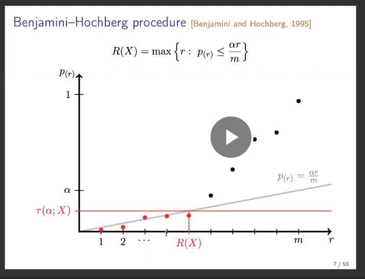
9.3 FDP / FDR and Benjamini-Hochberg

Setup:

• hypotheses $H_1,\dots ,H_m$,
• $p$-values $p_1,\dots ,p_m$ (not necessarily independent),
• rejected set $\mathcal{R}$ with $R=|\mathcal{R}|$,
• false rejections $V=|\mathcal{R}\cap {\mathcal{H}}_0|$.

Then

$$FDP=\frac{V}{R1},FDR=\mathbb{E}[FDP].$$

BH procedure at level $\alpha$:

1. Sort $p_{(1)}\le \cdots \le p_{(m)}$.
2. Reject up to $$R=\max \left\{r:p_{(r)}\le \frac{\alpha r}{m}\right\}.$$
3. Equivalent threshold rule: $$p_i\le \frac{\alpha R}{m}.$$

Adjusted BH $q$-value interpretation:

$$q_i=\min \{\alpha :H_i\text{ rejected by BH}(\alpha )\}.$$

10. Quantile Regression

Based on Koenker-style setup.

10.1 Conditional quantile function

Define conditional CDF

$$F_{Y\mid X}(y\mid x)=\mathbb{P}(Y\le y\mid X=x).$$

Conditional quantile at level $\tau$:

$$Q_{\tau }(Y\mid X=x)=F_{Y\mid X}^{-1}(\tau \mid x).$$

Linear quantile model:

$$Q_{\tau }(Y\mid X=x)=x^{\prime }{\beta }_{\tau }.$$

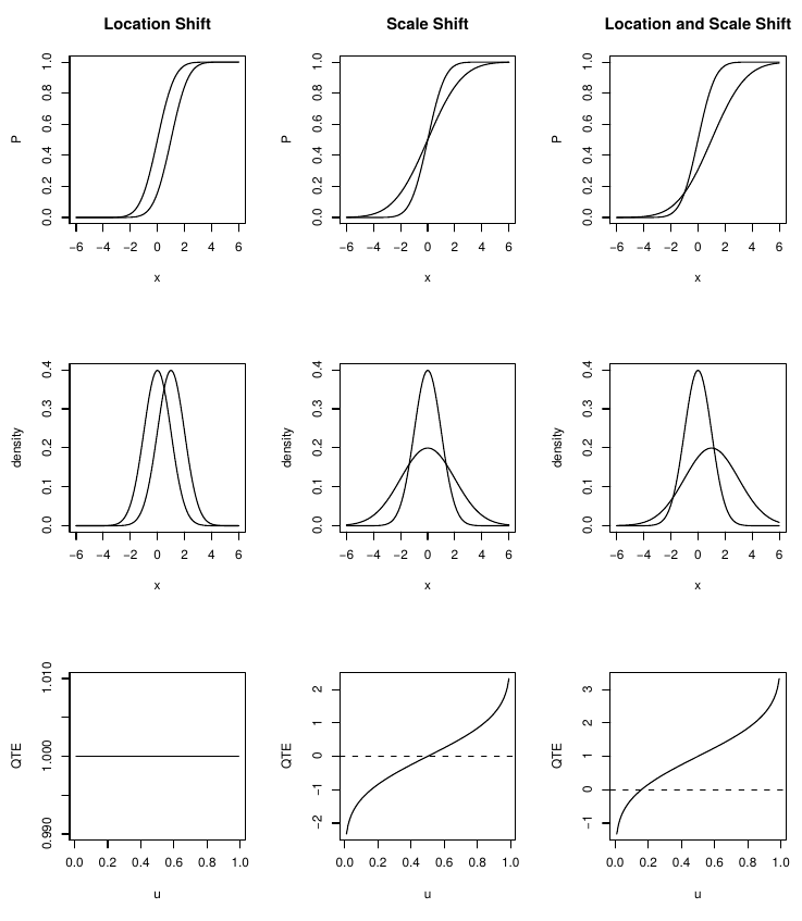
10.2 Relation to heteroskedasticity

If

$$Y_i=x_i^{\prime }\beta +{\epsilon }_i,{\epsilon }_i\mid x_i\sim \mathcal{N}(0,{\sigma }^2(x_i)),$$

then with $z_{\tau }$ standard-normal quantile,

$$Q_{\tau }(x_i)=x_i^{\prime }\beta +\sigma (x_i)z_{\tau }.$$

Thus quantile effects vary with $\tau$ when variance is covariate-dependent; under homoskedasticity, quantile slopes coincide across $\tau$.

10.3 Quantile-regression estimator

Check-loss objective:

$$\hat{\beta }(\tau )=\arg \underset{\beta \in {\mathbb{R}}^p}{\min }\sum _{i=1}^n{\rho }_{\tau }(y_i-x_i^{\prime }\beta ),$$

with

$${\rho }_{\tau }(u)=u(\tau -1\{u\le 0\}).$$

Equivalent split form:

$$Q_n({\beta }_{\tau })=\sum _{i:y_i\ge x_i^{\prime }\beta }\tau |y_i-x_i^{\prime }{\beta }_{\tau }|+\sum _{i:y_i<x_i^{\prime }\beta }(1-\tau )|y_i-x_i^{\prime }{\beta }_{\tau }|.$$

Asymptotic distribution in source notation:

$$\sqrt{N}({\hat{\beta }}_q-{\beta }_q)\stackrel{d}{\to }\mathcal{N}(0,A^{-1}B{A}^{-1}),$$

where

$$A=\mathrm{plim}\frac{1}{N}\sum _i{f}_{u_q}(0\mid x_i)x_i{x}_i^{\prime },B=\mathrm{plim}\frac{1}{N}\sum _{i}q(1-q)x_i{x}_i^{\prime }.$$

10.4 Lehmann-Doksum quantile treatment effect

Let $F$ be CDF of $Y_0$ (control) and $G$ be CDF of $Y_1$ (treated). Define horizontal shift $\Delta (x)$ via

$$F(x)=G(x+\Delta (x)).$$

Then

$$\delta (\tau )=G^{-1}(\tau )-F^{-1}(\tau )$$

is the QTE.

ATE from QTE:

$$\bar{\delta }={\int }_0^1\delta (\tau )d\tau =\mu (G)-\mu (F).$$

Empirical analogue:

$$\hat{\delta }(\tau )={\hat{G}}^{-1}(\tau )-{\hat{F}}^{-1}(\tau ).$$

Regression analogue:

$$Q_Y(\tau \mid D_i)=\alpha (\tau )+\delta (\tau )D_i.$$

10.5 Interpreting transformed quantile models

If monotone transform $h$ yields

$$Q_{h(Y)}(\tau \mid X=x)=h(Q_Y(\tau \mid X=x))=x^{\prime }\beta (\tau ),$$

then effects on $Q_Y$ follow via inverse-transform differentiation.

Example with log outcome: if modeling $Q_{\log Y}$, marginal effects on $Q_Y$ scale by $\exp (x^{\prime }\beta )$.

11. Measurement Error

11.1 Error in outcome variable

If observed $y=y^{\ast }+u_y$ and true model is $y^{\ast }=x\beta +\epsilon$, then observed regression is

$$y=x\beta +(\epsilon +u_y).$$

OLS slope remains unbiased if $u_y$ is orthogonal to $x$:

$$\mathrm{plim}\hat{\beta }=\frac{\mathrm{Cov}(y,x)}{\mathrm{Var}(x)}=\beta +\frac{\mathrm{Cov}(\epsilon +u_y,x)}{\mathrm{Var}(x)}=\beta .$$

Variance inflates because noise increases error variance.

11.2 Error in regressor (classical EIV)

If true regressor $X^{\ast }$ observed with error $X=X^{\ast }+V$ and

$$y=X^{\ast }\beta +U,$$

then observed equation has composite error correlated with $X$, so OLS is inconsistent.

Scalar attenuation result:

$$\mathrm{plim}\hat{\beta }=\frac{{\sigma }_{X^{\ast }}^2}{{\sigma }_{X^{\ast }}^2+{\sigma }_V^2}\beta ,$$

shrinking toward zero.

If measurement error ratio is $s={\sigma }_V^2/{\sigma }_{X^{\ast }}^2$, this reliability factor equals $1/(1+s)$.

11.3 Correlated regressors and measurement error

With correlated regressors, attenuation in one regressor can propagate bias into others and often worsens distortion.

11.4 IV remedy

If instrument $Z$ satisfies

$$\mathrm{Cov}(Z,X^{\ast })\ne 0,\mathrm{Cov}(Z,m)=0,$$

then in bivariate case

$${\hat{\beta }}_{IV}=\frac{\mathrm{Cov}(Y,Z)}{\mathrm{Cov}(X,Z)}=\beta .$$

12. Missing Data

Categories in source notes:

• MAR (missing at random): missingness may depend on other observables but not on the missing value itself, conditional on observables.
• MCAR (missing completely at random): observed sample is random subsample of full data.
• NMAR (not missing at random): neither MAR nor MCAR.

13. Inference on Functions of Parameters

13.1 Bootstrap

Core principle: resample from empirical CDF and recompute statistic to approximate its sampling distribution.

Algorithm:

1. From data $x_1,\dots ,x_N$, draw bootstrap sample $x_1^{\ast },\dots ,x_N^{\ast }$ (with replacement).
2. Compute statistic ${\hat{t}}^{\ast }=T(x_1^{\ast },\dots ,x_N^{\ast })$.
3. Repeat $B$ times.
4. Use empirical distribution of $\{{\hat{t}}_b^{\ast }{\}}_{b=1}^B$ for SEs/quantiles/bias correction.

Bootstrap SE:

$$s_{\hat{\theta },boot}^2=\frac{1}{B-1}\sum _{b=1}^B({\hat{\theta }}_b^{\ast }-{\bar{\hat{\theta }}}^{\ast }{)}^2,{\bar{\hat{\theta }}}^{\ast }=\frac{1}{B}\sum _{b=1}^B{\hat{\theta }}_b^{\ast }.$$

Bias logic:

$$\mathbb{E}[\hat{t}]-t_0\approx \mathbb{E}[\tilde{t}]-\hat{t}.$$

13.2 Edgeworth expansion intuition

For standardized mean,

$$\mathbb{P}\left(\frac{\sqrt{n}(\bar{X}-\mu )}{\sigma }\le \omega \right)=\Phi (\omega )+\varphi (\omega )\left[-\frac{\kappa }{6\sqrt{n}}({\omega }^2-1)+R_n\right],$$

with remainder term $R_n$ under regularity conditions.

13.3 Jackknife

Define leave-one-out estimates

$${\tilde{u}}_{-i}=T({\hat{F}}_{-i}),{\tilde{u}}_{(\cdot )}=\frac{1}{n}\sum _i{\tilde{u}}_{-i}.$$

A standard jackknife variance estimate is

$${\hat{\sigma }}_{jack}^2=\frac{n-1}{n}\sum _{i=1}^n({\tilde{u}}_{-i}-{\tilde{u}}_{(\cdot )}{)}^2.$$

13.4 Asymptotically pivotal statistics

A statistic is asymptotically pivotal if its limit distribution does not depend on unknown nuisance parameters.

13.5 Cluster wild bootstrap (few clusters)

Source algorithm (CGM style):

1. Estimate restricted model under null and get residuals ${\tilde{u}}_{ig}$.
2. For each bootstrap draw, assign each cluster $g$ a Rademacher weight $d_g\in \{-1,+1\}$.
3. Form pseudo-residuals $u_{ig}^{\ast }=d_g{\tilde{u}}_{ig}$ and pseudo-outcomes $$y_{ig}^{\ast }=x_{ig}^{\prime }{\tilde{\beta }}_{H_0}+u_{ig}^{\ast }.$$
4. Re-estimate unrestricted model on pseudo-data and compute test statistic $w_b^{\ast }$.
5. Bootstrap $p$-value from tail proportion of $|w_b^{\ast }|$ relative to observed $|w|$.

13.6 Delta method / propagation of error

If quantity of interest is

$$\hat{\theta }=f({\hat{\varphi }}_1,\dots ,{\hat{\varphi }}_p),$$

Taylor expansion gives variance propagation:

$$\mathrm{Var}(\hat{\theta })\approx \sum _{i=1}^p(f_i^{\prime }(\hat{\varphi }){)}^2\mathrm{Var}({\hat{\varphi }}_i)+2\sum _{i<j}{f}_i^{\prime }(\hat{\varphi })f_j^{\prime }(\hat{\varphi })\mathrm{Cov}({\hat{\varphi }}_i,{\hat{\varphi }}_j).$$

General vector form with $\tau =h(\beta )$:

$$\sqrt{n}(h(\hat{\beta })-h(\beta ))\stackrel{d}{\to }\mathcal{N}(0,\nabla h(\beta {)}^{\prime }\Sigma \nabla h(\beta )).$$

Scalar standardized form:

$$\frac{{\hat{\tau }}_n-\tau }{\widehat{se}({\hat{\tau }}_n)}\stackrel{d}{\to }\mathcal{N}(0,1),$$

with

$$\widehat{se}({\hat{\tau }}_n)=|g^{\prime }(\hat{\theta })|\widehat{se}({\hat{\theta }}_n).$$

13.7 Parametric bootstrap

Assume asymptotic parameter distribution is valid and simulate:

$${\beta }^{(m)}\sim \mathcal{N}({\beta }^{\ast },I_N(\beta {)}^{-1}),h^{(m)}=h({\beta }^{(m)}),$$

for $m=1,\dots ,M$, then summarize empirical distribution of $\{h^{(m)}\}$.

14. Generalized Method of Moments (GMM)

14.1 Linear GMM setup

Data $(Y_i,X_i,Z_i{)}_{i=1}^n$, with $Y_i\in \mathbb{R}$, $X_i\in {\mathbb{R}}^k$, instruments $Z_i\in {\mathbb{R}}^{\ell }$, and $\ell \ge k$.

Model:

$$Y_i=X_i^{\prime }\beta +U_i,\mathbb{E}[Z_i{U}_i]=0.$$

If just-identified ($k=\ell$):

$$\hat{\beta }={\left(\sum _i{Z}_i{X}_i^{\prime }\right)}^{-1}\sum _i{Z}_i{Y}_i.$$

Overidentified weighted criterion:

$$\hat{\beta }(W_n)=\arg \underset{b}{\min }{\left(\frac{1}{n}\sum _i{Z}_i(Y_i-X_i^{\prime }b)\right)}^{\prime }{W}_n\left(\frac{1}{n}\sum _i{Z}_i(Y_i-X_i^{\prime }b)\right).$$

14.2 General moment-condition formulation

Given moments

$$\mathbb{E}[g(W_i,{\theta }_0)]=0,$$

with $g\in {\mathbb{R}}^r$, $\theta \in {\mathbb{R}}^q$, $r\ge q$, define

$$g_n(\theta )=\frac{1}{n}\sum _{i}g(W_i,\theta ).$$

GMM objective:

$$\hat{\theta }=\arg \underset{\theta }{\min }{Q}_n(\theta ),Q_n(\theta )=g_n(\theta {)}^{\prime }{W}_n{g}_n(\theta ).$$

Jacobian:

$$D(\theta )=\mathbb{E}\left[\frac{\partial g(W_i,\theta )}{\partial {\theta }^{\prime }}\right].$$

Identification language:

• underidentified if rank$D<q$,
• just identified if rank$D=q$ and $r=q$,
• overidentified if $r>q$ with full rank for identified directions.

Asymptotic normality:

$$\sqrt{N}(\hat{\theta }-{\theta }_0)\stackrel{d}{\to }\mathcal{N}(0,V_{\theta }),$$ $$V_{\theta }=(D^{\prime }WD{)}^{-1}(D^{\prime }WSWD)(D^{\prime }WD{)}^{-1},$$

where

$$S=\mathbb{E}[g_i({\theta }_0)g_i({\theta }_0{)}^{\prime }].$$

14.3 Technical regularity conditions (summary)

The notes list standard requirements:

• compact parameter space,
• global identification,
• uniform LLN behavior of moments,
• continuity/differentiability of moment functions,
• finite moments,
• $W_n\stackrel{p}{\to }W$,
• interior true parameter.

14.4 Two-step efficient GMM

Variance-minimizing asymptotic weight is $W=S^{-1}$, giving

$$V_{\theta }=(D^{\prime }{S}^{-1}D{)}^{-1}.$$

Practical two-step algorithm:

1. Initialize $W_0=I$.
2. Compute preliminary ${\hat{\theta }}^{(1)}$.
3. Estimate $\hat{S}$ at ${\hat{\theta }}^{(1)}$.
4. Set $\hat{W}={\hat{S}}^{-1}$.
5. Re-optimize to get efficient ${\hat{\theta }}_{GMM}$.

14.5 Standard methods nested in GMM

• OLS moments: $g_i(\beta )=x_i(y_i-x_i^{\prime }\beta )$.
• IV/2SLS moments: $g_i(\beta )=z_i(y_i-x_i^{\prime }\beta )$.
• MLE moments: score equations $g_i(\theta )=\partial \log f(W_i;\theta )/\partial \theta$.

15. Empirical Likelihood and Generalized Empirical Likelihood

15.1 Nonparametric likelihood

For IID $X_1,\dots ,X_n$ with CDF $F$, nonparametric likelihood:

$$\mathcal{L}(F)=\prod _{i=1}^n(F(X_i)-F(X_i-)).$$

ECDF maximizes this criterion:

$$\hat{F}=\frac{1}{n}\sum _{i=1}^n{\delta }_{X_i}.$$

15.2 NPMLE as constrained optimization

Assign discrete masses $p_i$ on observed points and solve

$$\underset{p_1,\dots ,p_n}{\max }\frac{1}{n}\sum _{i=1}^n\log p_i\text{s.t.}\sum _i{p}_i=1.$$

Solution is ${\hat{p}}_i=1/n$.

15.3 Empirical likelihood with moment restrictions

Given moments

$$\mathbb{E}[m(W,{\theta }_0)]=0,$$

solve

$$\underset{p}{\max }\frac{1}{n}\sum _i\log p_i$$

subject to

$$\sum _i{p}_{i}m(W_i,\theta )=0,\sum _i{p}_i=1.$$

Lagrange multipliers $\lambda$ induce implicit equations for $(\hat{\theta },\hat{\lambda })$:

$$\frac{1}{n}\sum _i\frac{m(W_i,\hat{\theta })}{1+{\hat{\lambda }}^{\prime }m(W_i,\hat{\theta })}=0,$$

plus corresponding score equation in $\theta$.

Dual saddlepoint form:

$$\underset{\theta \in \Theta }{\max }\underset{\lambda }{\min }\frac{1}{n}\sum _i\left[-\log (1+{\lambda }^{\prime }m(W_i,\theta ))\right].$$

15.4 Generalized empirical likelihood (GEL)

Replace log criterion with shape-constrained $\rho (v)$ satisfying normalizations at 0:

$$\underset{\theta \in \Theta }{\min }\underset{\lambda \in {\Lambda }_n}{\sup }\frac{1}{n}\sum _i\rho ({\lambda }^{\prime }m(W_i,\theta )).$$

Special cases in notes:

• $\rho (v)=\log (1-v)$ gives EL,
• $\rho (v)=-\frac{1}{2}{v}^2-v$ gives CUE,
• $\rho (v)=1-e^v$ gives exponential tilting.

Primal formulation uses Cressie-Read divergence family for weights.

16. M-estimation

M-estimator solves

$$\sum _{i=1}^n\psi (O_i,\hat{\theta })=0,$$

with i.i.d. observations $O_i$ and estimating function $\psi$.

Asymptotic sandwich variance:

$$\mathrm{Var}(\hat{\theta })\approx B_n^{-1}{M}_n(B_n^{-1}{)}^{\prime },$$

where

$$B_n=\frac{1}{n}\sum _i-{\psi }_i^{\prime }(\hat{\theta })\text{(bread)},$$ $$M_n=\frac{1}{n}\sum _i{\psi }_i(\hat{\theta }){\psi }_i(\hat{\theta }{)}^{\prime }\text{(meat)}.$$

This framework nests many estimators. For MLE, $\psi$ is the score.

Related notes

• index
• probability-and-mathstats
• long_squiggly_permutation
• 2025-09-29