Augmented Balancing for Panel Data

Combine an untreated-outcome model with unit and time balancing

AugmentedBalancing estimates panel ATT by adding balancing corrections to a supplied untreated-outcome surface. The outcome model and the balancing weights solve different problems: the outcome model supplies a first counterfactual prediction, while unit and time weights correct systematic residual discrepancies between treated units and never-treated donors.

The estimator uses the matrix-first panel API:

fit(Y, W, outcome_model=None)

Y is an (n_units, n_periods) balanced outcome matrix. W is a same-shaped binary absorbing-treatment matrix. The optional outcome_model must contain untreated-outcome predictions for the entire panel. It should be estimated without using treated post-treatment outcomes.

This vignette builds a staggered-adoption panel, fits a low-rank nuisance surface with MatrixCompletion, and compares outcome-only, balancing-only, and augmented specifications. See the AugmentedBalancing API page for the complete constructor, output schema, and estimator formula.

1 Simulate A Staggered Factor Panel

import matplotlib.pyplot as plt
import numpy as np
import pandas as pd

import crabbymetrics as cm

np.set_printoptions(precision=4, suppress=True)

The untreated surface combines unit effects, common time effects, and three latent factors. Eight treated units adopt in two cohorts. Treatment effects increase with exposure duration and vary modestly across units.

rng = np.random.default_rng(611)

n_control = 48
n_treated = 8
n_periods = 30
n_units = n_control + n_treated
period = np.arange(n_periods)

factors = np.vstack(
    [
        np.sin(np.linspace(0.0, 2.6 * np.pi, n_periods)),
        np.cos(np.linspace(0.0, 1.4 * np.pi, n_periods)),
        (period - period.mean()) / n_periods,
    ]
)
loadings = rng.normal(size=(n_units, factors.shape[0]))
unit_effects = rng.normal(scale=0.6, size=n_units)
time_effects = 0.035 * period + 0.25 * np.sin(period / 4.0)

Y0 = (
    unit_effects[:, None]
    + time_effects[None, :]
    + loadings @ factors
    + rng.normal(scale=0.10, size=(n_units, n_periods))
)
Y = Y0.copy()
W = np.zeros_like(Y)

treated_units = np.arange(n_control, n_units)
cohort_starts = np.r_[np.repeat(18, 4), np.repeat(23, 4)]
for offset, (unit, start) in enumerate(zip(treated_units, cohort_starts)):
    effect_path = 0.7 + 0.04 * np.arange(n_periods - start) + 0.05 * (offset - 3.5)
    W[unit, start:] = 1.0
    Y[unit, start:] += effect_path

true_att = float((Y - Y0)[W == 1.0].mean())
print("panel shape:", Y.shape)
print("treated cohorts:", np.unique(cohort_starts))
print("never-treated donors:", n_control)
print("treated cells:", int(W.sum()))
print("true ATT:", round(true_att, 4))

panel shape: (56, 30)
treated cohorts: [18 23]
never-treated donors: 48
treated cells: 76
true ATT: 0.8568

The estimator infers treated units, adoption cohorts, event time, and never-treated donors from W. Units treated in the first panel period are invalid because they have no pre-treatment history; nonabsorbing treatment paths are also rejected.

2 Fit An Untreated-Outcome Surface

AugmentedBalancing deliberately does not own nuisance estimation. Any finite same-shaped prediction matrix can be supplied. Here MatrixCompletion estimates a low-rank surface using cells with W == 0; treated post-treatment cells are excluded from its fitting objective.

outcome_fit = cm.MatrixCompletion(
    lambda_fraction=0.12,
    fit_unit_effects=True,
    fit_time_effects=True,
    max_iterations=500,
    tolerance=1e-6,
)
outcome_fit.fit(Y, W)
outcome_model = np.asarray(outcome_fit.predict())
outcome_summary = outcome_fit.summary()

print("outcome-model ATT:", round(float(outcome_summary["att"]), 4))
print("outcome-model converged:", outcome_summary["converged"])
print("outcome-model iterations:", outcome_summary["iterations"])

outcome-model ATT: 0.668
outcome-model converged: True
outcome-model iterations: 14

In an empirical workflow, nuisance fitting should respect the assignment design and should not leak treated post-treatment outcomes. Cross-fitting, tuning, and uncertainty propagation remain the analyst’s responsibility.

3 Compare The Estimator Family

One class spans several familiar estimators. Omitting outcome_model sets the nuisance surface to zero. Supplying it turns the same balancing correction into an augmented estimator.

specifications = {
    "Outcome model only": (
        dict(balance="none"),
        outcome_model,
    ),
    "Unit balancing": (
        dict(balance="unit", zeta_omega=0.03),
        None,
    ),
    "Double balancing": (
        dict(balance="double", zeta_omega=0.03, zeta_lambda=0.01),
        None,
    ),
    "Augmented double": (
        dict(
            balance="double",
            balance_on="residual",
            zeta_omega=0.03,
            zeta_lambda=0.01,
        ),
        outcome_model,
    ),
}

fits = {}
rows = []
for name, (options, nuisance) in specifications.items():
    model = cm.AugmentedBalancing(**options, max_iterations=2000)
    model.fit(Y, W, nuisance)
    summary = model.summary()
    fits[name] = (model, summary)
    estimate = float(summary["att"])
    rows.append(
        {
            "Specification": name,
            "ATT": estimate,
            "Absolute error": abs(estimate - true_att),
            "Pre-period RMSE": float(summary["pre_rmse"]),
        }
    )

comparison = pd.DataFrame(rows).set_index("Specification")
comparison.loc["Truth", ["ATT", "Absolute error"]] = [true_att, 0.0]
comparison.round(4)

	ATT	Absolute error	Pre-period RMSE
Specification
Outcome model only	0.6680	0.1888	0.0839
Unit balancing	0.8173	0.0396	0.2912
Double balancing	0.8268	0.0300	0.2912
Augmented double	0.8087	0.0482	0.0509
Truth	0.8568	0.0000	NaN

balance="unit" optimizes donor weights and uses uniform pre-period weights. balance="time" does the reverse. balance="double" optimizes both dimensions. With balance_on="residual", the weight problems match Y - outcome_model; with balance_on="raw", they match Y but still apply the resulting correction to outcome-model residuals.

The comparison is diagnostic, not a theorem that augmentation must dominate every balancing-only estimator in every realized sample. Its advantage is architectural: a useful outcome model can absorb broad structure while balancing targets remaining residual discrepancies.

4 Inspect Counterfactuals And Event Time

predict() returns the fitted untreated counterfactual matrix and treatment_effect() returns Y - predict(). Rows for never-treated donors are NaN because the estimator targets treated-unit counterfactuals.

augmented_model, augmented = fits["Augmented double"]
counterfactual = np.asarray(augmented_model.predict())
effects = np.asarray(augmented_model.treatment_effect())

print("counterfactual shape:", counterfactual.shape)
print("effect shape:", effects.shape)
print("finite donor counterfactual cells:", np.isfinite(counterfactual[:n_control]).sum())
print("estimated ATT:", round(float(augmented["att"]), 4))

counterfactual shape: (56, 30)
effect shape: (56, 30)
finite donor counterfactual cells: 0
estimated ATT: 0.8087

The weighted event-study summary aggregates cohort-specific effects using the number of treated observations represented by each row.

event = augmented["event_study"]["weighted"]
event_time = np.asarray(event["event_time"])
event_estimate = np.asarray(event["estimate"])

unit = treated_units[0]
start = cohort_starts[0]

fig, axes = plt.subplots(1, 2, figsize=(12.5, 4.4), constrained_layout=True)

axes[0].plot(period, Y[unit], color="black", lw=2.0, label="Observed")
axes[0].plot(period, Y0[unit], color="#1b9e77", lw=2.0, label="True untreated")
axes[0].plot(period, counterfactual[unit], color="#7570b3", lw=2.0, label="Estimated untreated")
axes[0].axvline(start, color="0.45", ls="--", lw=1.0)
axes[0].set_title(f"Counterfactual Path For Unit {unit}")
axes[0].set_xlabel("Period")
axes[0].set_ylabel("Outcome")
axes[0].legend(frameon=False)

axes[1].plot(event_time, event_estimate, marker="o", color="#7570b3", label="Estimated")
true_event = []
for event_value in event_time.astype(int):
    mask = np.zeros_like(W, dtype=bool)
    for treated_unit, treated_start in zip(treated_units, cohort_starts):
        target_period = treated_start + event_value
        if 0 <= target_period < n_periods:
            mask[treated_unit, target_period] = True
    true_event.append(float((Y - Y0)[mask].mean()))
axes[1].plot(event_time, true_event, marker="s", color="#1b9e77", label="Truth")
axes[1].axhline(0.0, color="0.55", lw=1.0)
axes[1].axvline(0.0, color="0.45", ls="--", lw=1.0)
axes[1].set_title("Treated-Count-Weighted Event Study")
axes[1].set_xlabel("Period Relative To Treatment")
axes[1].set_ylabel("Effect")
axes[1].legend(frameon=False)

plt.show()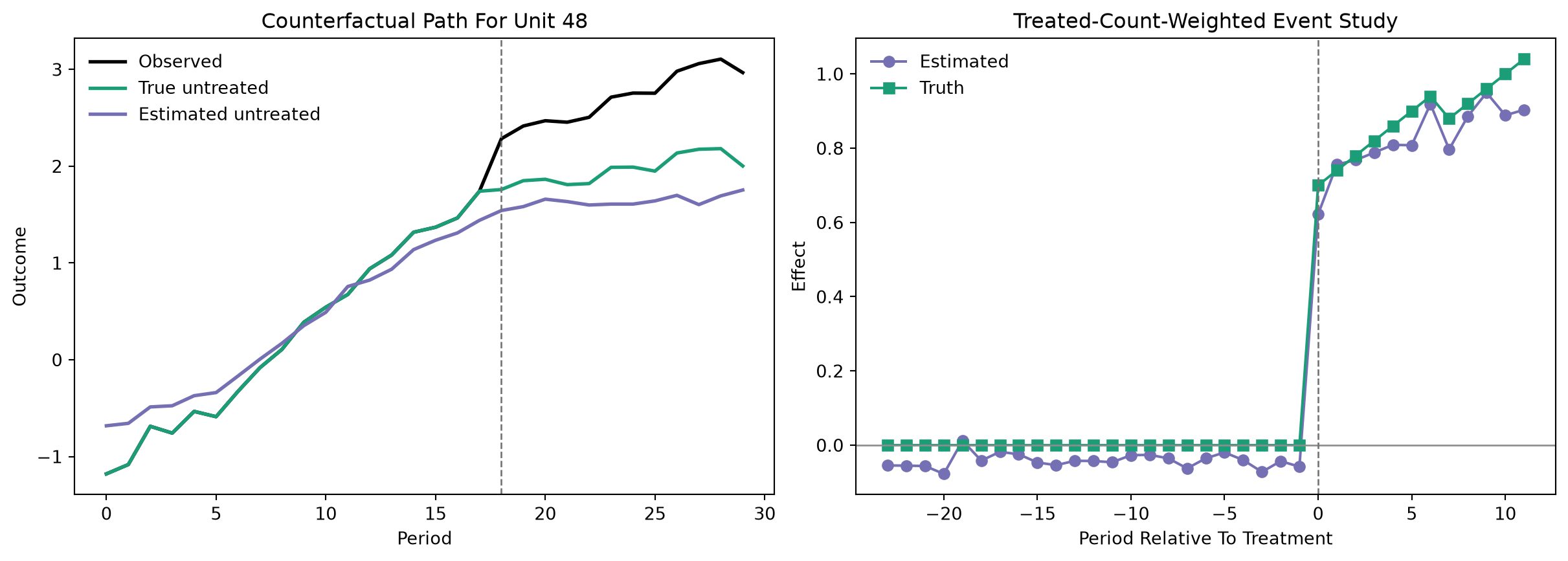

Pre-treatment event-time estimates are placebo-style fit diagnostics, not causal effects. Large pre-period discrepancies indicate that the outcome surface and balancing weights do not reproduce treated histories well.

5 Read Weight Targets Correctly

With the default unit_target="cohort", each row of unit_weights belongs to one adoption cohort. With time_target="all", each row of time_weights belongs to one cohort and targets its average post-period donor outcome. Mapping arrays make these row semantics explicit.

control_units = np.asarray(augmented["control_units"])
unit_weights = np.asarray(augmented["unit_weights"])
time_weights = np.asarray(augmented["time_weights"])

weight_rows = pd.DataFrame(
    {
        "cohort": augmented["target_cohorts"],
        "target_unit": augmented["target_units"],
        "unit_weight_sum": unit_weights[:, control_units].sum(axis=1),
        "zeta_omega": augmented["zeta_omega"],
    }
)
time_rows = pd.DataFrame(
    {
        "cohort": augmented["time_target_cohorts"],
        "target_period": augmented["time_target_periods"],
        "time_weight_sum": time_weights.sum(axis=1),
        "zeta_lambda": augmented["zeta_lambda"],
    }
)

display(weight_rows.round(6))
display(time_rows.round(6))

	cohort	target_unit	unit_weight_sum	zeta_omega
0	18	-1	1.0	0.03
1	23	-1	1.0	0.03

	cohort	target_period	time_weight_sum	zeta_lambda
0	18	-1	1.0	0.01
1	23	-1	1.0	0.01

target_unit == -1 denotes a cohort-average target. time_target_period == -1 denotes one all-post target. Set unit_target="individual" for one donor vector per treated unit and time_target="period" for one time-weight vector per post-treatment period. Those choices are more flexible but can be noisier and substantially increase the number of optimization problems.

6 Practical Specification Guidance

• Start with balance="double", unit_target="cohort", and time_target="all" when the target is an aggregate ATT and treated cohorts have several units.
• Supply a nuisance surface when a defensible untreated-outcome model is available. Use balance_on="residual" when weights should explicitly target what that model fails to explain.
• Use unit_target="individual" when treated units need materially different donor mixtures. Use time_target="period" when post-period-specific time matching is substantively important.
• Compare pre_rmse, inspect pre-treatment event-time gaps, and examine weight concentration. A numerically converged simplex solve is not evidence of a credible comparison design.
• unit_loss="penalized_scm" switches the donor problem to the standardized penalized-SCM loss. Its unit_penalty is separate from the SDID-style ridge scale zeta_omega.
• The class does not provide standard errors, confidence intervals, nuisance cross-fitting, or tuning selection. Inference must reflect both panel dependence and the way the nuisance surface and weights were estimated.