Conditional moments: kernels and sieves

Estimate a response function from instrument restrictions rather than prediction error.

Why not regress the outcome on the treatment?

Consider Y=h_0(T)+U, with E[U\mid Z]=0 but potentially E[U\mid T]\ne0. Ordinary prediction learns E[Y\mid T], not necessarily h_0. An instrument restriction instead asks whether the fitted residual is orthogonal to every function of Z. Identification still requires enough variation in the instruments: a flexible optimizer cannot supply completeness or instrument validity.

Trex connects a differentiable torch.nn.Module for h_\theta to a moment callback \rho_\theta=\rho(h_\theta(T),Y). For an IV regression, use \rho_\theta=h_\theta(T)-Y. Both estimators below operate on the complete sample; they are not stochastic-minibatch IV estimators.

Two finite-sample objectives

Maximum moment restriction (MMR) uses a positive-definite kernel:

Q_K(\theta)=\frac{1}{n^2}\sum_{i,j} \rho_{\theta,i}'\rho_{\theta,j} k(Z_i,Z_j).

Trex uses an RBF kernel, with a median-distance bandwidth when none is given. This is the nonnegative, diagonal-including quadratic criterion, not an unbiased off-diagonal U-statistic. The kernel matrix costs O(n^2) memory. For vector-valued moments the objective sums the componentwise quadratic forms. Instrument scaling and bandwidth affect the criterion’s geometry.

Sieve minimum distance (SMD) replaces all instrument functions by a finite polynomial basis B_i=b(Z_i):

M_\theta=n^{-1}\sum_i B_i\rho_{\theta,i}',\qquad Q_B(\theta)=\operatorname{tr}\left[ M_\theta'(n^{-1}B'B+rI)^+M_\theta\right].

Trex standardizes instruments before constructing the polynomial sieve. degree, interactions, and the ridge r determine the approximation. Increasing the degree can add weak or nearly redundant moments; it is not a free improvement in identification.

Worked example: an endogenous nonlinear regressor

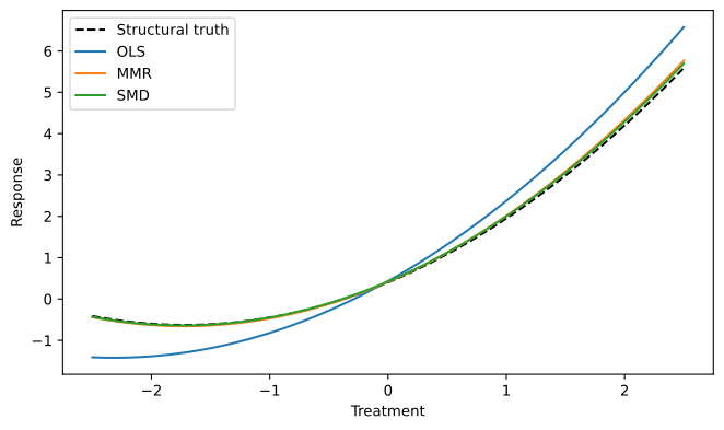
Here T=0.9Z+V and U=0.7V+\varepsilon. We know the response is quadratic and estimate its coefficients. This deliberately separates the instrument problem from neural-network approximation and local minima.

import numpy as np
import pandas as pd
import torch
import matplotlib.pyplot as plt
from trex import MaximumMomentRestriction, SieveMinimumDistance

torch.set_num_threads(1)
torch.manual_seed(721)
n = 700
z = torch.randn(n, 1, dtype=torch.float64)
v = torch.randn_like(z)
t = 0.9 * z + v
y = 0.4 + 1.2*t + 0.35*t.square() + 0.7*v + 0.3*torch.randn_like(z)

class Quadratic(torch.nn.Module):
    def __init__(self):
        super().__init__()
        self.beta = torch.nn.Parameter(torch.zeros(3, dtype=torch.float64))

    def forward(self, t):
        return self.beta[0] + self.beta[1]*t + self.beta[2]*t.square()

fits = {}
for name, cls, options in [
    ("MMR", MaximumMomentRestriction, {}),
    ("SMD", SieveMinimumDistance, {"degree": 3}),
]:
    fits[name] = cls(
        model=Quadratic(), moment_function=lambda pred, y: pred-y,
        device="cpu", dtype=torch.float64, maxiter=80, **options,
    ).fit(t, y, z)

design = torch.cat([torch.ones_like(t), t, t.square()], dim=1)
ols = torch.linalg.lstsq(design, y).solution[:, 0].numpy()
coefficients = {"Truth": [0.4, 1.2, 0.35], "OLS": ols}
coefficients.update({name: fit.model.beta.detach().numpy() for name, fit in fits.items()})
pd.DataFrame(coefficients, index=["Intercept", "Linear", "Quadratic"]).round(3)

	Truth	OLS	MMR	SMD
Intercept	0.40	0.433	0.411	0.422
Linear	1.20	1.598	1.241	1.226
Quadratic	0.35	0.344	0.360	0.353

grid = torch.linspace(-2.5, 2.5, 150, dtype=torch.float64)[:, None]
fig, ax = plt.subplots()
ax.plot(grid[:, 0], 0.4+1.2*grid[:, 0]+0.35*grid[:, 0]**2, "k--", label="Structural truth")
ax.plot(grid[:, 0], ols[0]+ols[1]*grid[:, 0]+ols[2]*grid[:, 0]**2, label="OLS")
for name, fit in fits.items():
    ax.plot(grid[:, 0], fit.predict(grid).detach().numpy().ravel(), label=name)
ax.set(xlabel="Treatment", ylabel="Response"); ax.legend(); plt.show()

Figure 1: The structural curve and fits. OLS targets a different conditional expectation because treatment is endogenous.

Diagnostics and scope

Inspect the fitted criterion and loss history, and evaluate moments on new observations. A small training loss can mean overfitting the instrument sample. Compare sensitivity to bandwidth or sieve degree on validation moments rather than selecting by in-sample loss alone. The hsic helper is a dependence diagnostic, not a replacement for an identification argument.

These classes do not supply a complete inferential procedure for learned functions. Their interfaces accept neural modules, but neither automatic standard errors nor causal validity follows from that flexibility. Account for regularization, approximation, weak instruments, and tuning in any inferential extension. For finite-dimensional unconditional moments and sandwich covariances, see GMM.

API: MaximumMomentRestriction, SieveMinimumDistance, mmr_loss, polynomial_sieve.