Latent-factor generalized linear models

Interactive effects with covariates, masks, offsets, and non-Gaussian responses.

Interactive rather than additive heterogeneity

An additive unit effect shifts every period equally. Interactive effects allow units to respond differently to common shocks:

\eta_{it}=X_{it}'\beta+A_i'B_t+o_{it},\qquad E[Y_{it}\mid X,A,B]=g^{-1}(\eta_{it}).

LatentFactorGLM supports Gaussian/identity, Bernoulli/logit and Poisson/log families. The offset o_{it} is known, not estimated. Unit and time IDs index factor rows. The model does not automatically add separate unit and time intercepts: represent desired additive terms explicitly or choose an appropriate model specification.

Trex minimizes the mean observed-cell negative log likelihood, plus

\frac{\lambda}{2}\{\operatorname{mean}(A^2)+\operatorname{mean}(B^2)\} +\frac{\lambda_\beta}{2}\operatorname{mean}(\beta^2).

The Gaussian loss is half the squared error. The factorization makes optimization nonconvex; factor rescalings and rotations also make individual factor coordinates non-unique. Interpret the product AB' or predicted means, not an arbitrary fitted axis as an identified economic trait.

Worked example: Gaussian panel with masked cells

import numpy as np
import pandas as pd
import torch
import matplotlib.pyplot as plt
from trex import LatentFactorGLM

torch.set_num_threads(1)
torch.manual_seed(403)
N, T = 35, 20
X = torch.randn(N, T, 2, dtype=torch.float64)
beta = torch.tensor([0.9, -0.6], dtype=torch.float64)
A = torch.randn(N, 2, dtype=torch.float64)*0.6
B = torch.randn(T, 2, dtype=torch.float64)*0.6
offset = 0.1*torch.randn(N, T, dtype=torch.float64)
mean = X @ beta + A @ B.T + offset
y = mean + 0.1*torch.randn_like(mean)
mask = torch.rand(N, T) < 0.8
fit = LatentFactorGLM(
    family="gaussian", rank=2, penalty=1e-3,
    optimizer_kwargs={"lr": 0.04, "weight_decay": 0.0},
    maxiter=1400, tol=1e-8, device="cpu",
).fit(X, y, mask=mask, offset=offset)
pred = fit.predict_mean(X, offset=offset).detach()
pd.DataFrame({"Truth": beta.numpy(), "Estimate": fit.params["coef"].numpy()},
             index=["x1", "x2"]).round(4)

	Truth	Estimate
x1	0.9	0.8957
x2	-0.6	-0.5950

fig, ax = plt.subplots()
ax.scatter(mean[~mask].numpy(), pred[~mask].numpy(), alpha=0.6, s=16)
ax.plot([-3, 3], [-3, 3], "k--")
ax.set(xlabel="True conditional mean", ylabel="Fitted mean")
plt.show()
print("Held-out RMSE against noisy outcomes:", float(((pred[~mask]-y[~mask])**2).mean().sqrt()))

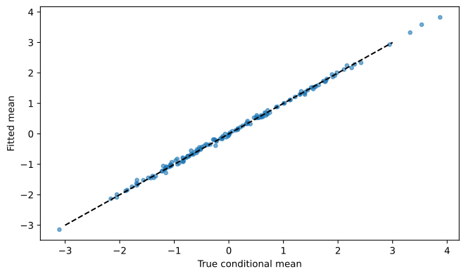
Figure 1: Predictions for held-out cells. The diagonal represents exact prediction of the latent conditional mean.

Held-out RMSE against noisy outcomes: 0.11158441136709693

Binary and count outcomes

Changing the family changes the likelihood and inverse link, not merely a post-processing transform of a least-squares fit. Here is a rank-zero Poisson fit, a useful reference case for the nonlinear implementation.

torch.manual_seed(404)
count_X = torch.ones(N, T, 2, dtype=torch.float64)
count_X[:, :, 1] = torch.randn(N, T, dtype=torch.float64)*0.5
exposure = 0.7 + torch.rand(N, T, dtype=torch.float64)
count_beta = torch.tensor([-0.2, 0.4], dtype=torch.float64)
count_y = torch.poisson(torch.exp(count_X @ count_beta) * exposure)
count_fit = LatentFactorGLM(
    family="poisson", rank=0, penalty=0,
    optimizer_kwargs={"lr": 0.04, "weight_decay": 0.0},
    maxiter=800, tol=1e-8, device="cpu",
).fit(count_X, count_y, offset=exposure.log())
print("Poisson coefficients:", count_fit.params["coef"].numpy().round(3))
print("Mean fitted count:", float(count_fit.predict_mean(count_X, offset=exposure.log()).mean()))

Poisson coefficients: [-0.206  0.341]
Mean fitted count: 1.0108175447360908

For Bernoulli responses choose family="bernoulli" and call predict_proba. For either family, predict_index returns \eta, whereas predict_mean applies the inverse link. Trex caps very large log rates in Poisson prediction for numerical safety; inspect extreme-index fits rather than treating saturation as evidence of a well-behaved model.

Layout and limitations

Dense input uses X.shape == (N,T,p) and y.shape == (N,T). An observation list uses (n_obs,p) and explicit unit_ids and time_ids. A boolean mask selects training observations in either layout; predictions still require levels represented in the fitted model. This is not a cold-start embedding model for new units or dates.

Use multiple starts and time- or block-aware validation for rank and penalty. The current implementation does not report identification-aware coefficient or treatment-effect covariance estimates. With short panels, nonlinear incidental parameters can matter. Interactive effects are a model for unobserved heterogeneity, not by themselves a causal identification strategy.

API: LatentFactorGLM. Related: matrix completion, fixed-effect GLMs.