Dynamic choice: NFXP and CCP inversion

Estimate a replacement problem, solve its Bellman equation, and change a policy.

Why current utility is not enough

A decision changes both current utility and the distribution of future states. Let P_a(s,s') be a controlled transition matrix, u_\theta(s,a) flow utility, and \delta<1 the discount factor. Under independent type-I extreme-value choice shocks, a normalized integrated value function satisfies

V_\theta(s)=\log\sum_a\exp\left[u_\theta(s,a)+ \delta\sum_{s'}P_a(s,s')V_\theta(s')\right].

The Euler constant is absorbed into a common value normalization; it does not affect choice probabilities. The softmax of the choice-specific values gives p_\theta(a\mid s). A discount factor below one makes this Bellman map a contraction. Trex uses dense transition tensors of shape (n_states, n_choices, n_states).

Two estimation routes

RustNFP maximizes \sum_i\log p_\theta(a_i\mid s_i), solving the Bellman fixed point inside likelihood evaluations. Stable log probabilities matter: adding a probability floor before taking logs can flatten gradients for very unlikely observations.

HotzMillerCCP first estimates conditional choice probabilities \hat p. With P_{\hat p}=\sum_a\hat p_aP_a, policy evaluation gives

(I-\delta P_{\hat p})V_\theta =\sum_a\hat p_a u_\theta(s,a)-\sum_a\hat p_a\log\hat p_a.

This avoids repeated Bellman iterations during the second-stage criterion. Estimated CCPs still introduce sampling error. Sparse state-action cells, smoothing, and first-stage approximation can strongly affect results. Trex’s post-fit predict_proba re-solves the structural model rather than returning the empirical first-stage probabilities.

Worked example: replace a deteriorating machine

Keeping the machine costs \theta_m s; replacement costs \theta_r. Replacement mostly resets the state. We generate decisions from an independent NumPy Bellman calculation, hold the transition law fixed, and estimate both cost parameters. This is a small correctness illustration, not Rust’s original bus data or an empirical demand estimate.

import numpy as np
import pandas as pd
import torch
import matplotlib.pyplot as plt
from scipy.special import logsumexp, softmax
from trex.choice import RustNFP, HotzMillerCCP, ReplacementUtility, DynamicChoiceData

torch.set_num_threads(1)
rng = np.random.default_rng(604)
S, discount = 8, 0.9
P = np.zeros((S, 2, S))
for s in range(S):
    P[s, 0, s] += 0.25
    P[s, 0, min(s+1, S-1)] += 0.75
    P[s, 1, 0], P[s, 1, 1] = 0.8, 0.2
truth = np.array([0.12, 2.0])
u = np.c_[-truth[0]*np.arange(S), np.full(S, -truth[1])]
value = np.zeros(S)
for _ in range(1000):
    new = logsumexp(u + discount*np.einsum("sat,t->sa", P, value), axis=1)
    if np.max(np.abs(new-value)) < 1e-12:
        value = new
        break
    value = new
prob = softmax(u + discount*np.einsum("sat,t->sa", P, value), axis=1)
rows = []
for individual in range(160):
    state = int(rng.integers(S))
    for time in range(45):
        action = int(rng.choice(2, p=prob[state]))
        next_state = int(rng.choice(S, p=P[state, action]))
        rows.append((state, action, next_state, individual, time))
        state = next_state
columns = torch.tensor(np.array(rows), dtype=torch.long).T
data = DynamicChoiceData(*columns)
models = {}
for name, cls in [("NFXP", RustNFP), ("CCP", HotzMillerCCP)]:
    model = cls(S, 2, discount, maxiter=120, tol=1e-8, device="cpu")
    model.set_transition_probabilities(torch.tensor(P))
    model.set_flow_utility(ReplacementUtility(device="cpu"))
    model.fit(data, init_params=torch.tensor([0.1, 1.8], dtype=torch.float64))
    models[name] = model
pd.DataFrame({"Truth": truth, **{name: m.params["coef"].detach().numpy()
                                 for name, m in models.items()}},
             index=["Maintenance cost", "Replacement cost"]).round(4)

	Truth	NFXP	CCP
Maintenance cost	0.12	0.1101	0.1100
Replacement cost	2.00	1.9622	1.9621

A policy counterfactual

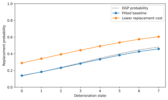
Reducing replacement cost changes continuation values as well as current utility. counterfactual re-solves the model and can simulate new paths without mutating fitted baseline parameters. It starts each individual at their earliest observed state. Supply an explicit horizon for an unbalanced panel.

model = models["NFXP"]
states = torch.arange(S)
baseline = model.predict_proba(states).detach().numpy()
old_coef = model.params["coef"].clone()
cf = model.counterfactual(
    data, {"theta_replacement_cost": float(old_coef[1])*0.5},
    rng=torch.Generator().manual_seed(70), n_periods=20,
)
changed = cf["counterfactual_probs"].detach().numpy()
assert torch.equal(old_coef, model.params["coef"])
fig, ax = plt.subplots()
ax.plot(np.arange(S), prob[:, 1], "k:", label="DGP probability")
ax.plot(np.arange(S), baseline[:, 1], "o-", label="Fitted baseline")
ax.plot(np.arange(S), changed[:, 1], "o-", label="Lower replacement cost")
ax.set(xlabel="Deterioration state", ylabel="Replacement probability", ylim=(0, 1))
ax.legend(); plt.show()

Figure 1: Structural replacement probabilities before and after reducing replacement cost by half.

What this does not establish

The example conditions on known transitions and a fixed discount factor. If transitions are estimated, their uncertainty belongs in inference. Utility levels and the shock scale require normalization; a good fit to a policy does not identify unrestricted rewards or all counterfactuals. LinearFlowUtility supports specified features, while DeepValueFunction is a helper, not a turnkey neural inverse-RL estimator.

Standard errors for the dynamic estimators are not implemented. Dense transition storage also limits large state spaces. Check Bellman residuals, state coverage, likelihood gradients and optimizer sensitivity before using the results in a structural application.

API: RustNFP, HotzMillerCCP, DynamicChoiceData, ReplacementUtility, estimate_transition_matrix.