Learning a robust regression score

Antitonic score estimation and a convex residual loss.

From a density to an estimating equation

For a location regression Y=X'\beta+\varepsilon with density f, let \psi(e)=\partial_e\log f(e). The likelihood equation is \sum_i X_i\psi(Y_i-X_i'\beta)=0. A Gaussian density gives a linear score and least squares. Other error shapes suggest different weighting of large residuals, but estimating an unrestricted density derivative can be unstable.

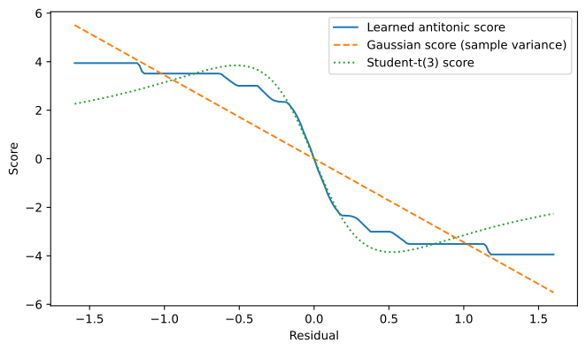
Trex estimates a decreasing (antitonic) score. If \rho'(e)=-\psi(e), then a decreasing score makes \rho convex. This is a shape restriction on the score, not a claim that every heavy-tailed density has a decreasing score. In particular, the exact Student-t score is not globally decreasing.

What the implementation does

AntitonicScoreMatchingRegression starts from a least-squares or LAD pilot. It smooths residuals with a kernel density estimate, constructs a score using the estimated density on a quantile grid, applies a pooled-adjacent-violators monotonicity projection, and interpolates the resulting score. It alternates score estimation with regression updates a chosen number of times.

The symmetry option imposes an odd score. It is useful for symmetric errors, but can be inappropriate for skewed disturbances. bandwidth, k, and kernel_grid_size control density smoothing and numerical resolution. This estimator uses NumPy/SciPy on the CPU despite sharing the Trex interface.

Worked example: Student-t disturbances

import numpy as np
import pandas as pd
import matplotlib.pyplot as plt
from trex import AntitonicScoreMatchingRegression

rng = np.random.default_rng(144)
n = 450
X = rng.normal(size=(n, 2))
truth = np.array([0.4, 1.5, -0.75])
errors = 0.3 * rng.standard_t(3, size=n)
y = truth[0] + X @ truth[1:] + errors
fit = AntitonicScoreMatchingRegression(
    pilot="lad", symmetric=True, alt_iter=2, k=500,
    kernel_grid_size=1024, max_iter=60, device="cpu",
).fit(X, y)
ols = np.linalg.lstsq(np.c_[np.ones(n), X], y, rcond=None)[0]
pd.DataFrame({"Truth": truth, "OLS": ols, "Antitonic": fit.beta_,
              "Reported SE": fit.std_errors_},
             index=["Intercept", "x1", "x2"]).round(4)

	Truth	OLS	Antitonic	Reported SE
Intercept	0.40	0.3911	0.3866	0.0191
x1	1.50	1.5299	1.5253	0.0186
x2	-0.75	-0.7935	-0.7502	0.0194

Unlike LinearRegression, this estimator adds an intercept by default. coef_ contains slopes and beta_ includes the intercept. Do not also add a constant column unless fit_intercept=False.

grid = np.linspace(-1.6, 1.6, 200)
fig, ax = plt.subplots()
ax.plot(grid, fit.score_(grid), label="Learned antitonic score")
ax.plot(grid, -grid/np.var(errors), "--", label="Gaussian score (sample variance)")
ax.plot(grid, -4*grid/(3*0.3**2+grid**2), ":", label="Student-t(3) score")
ax.set(xlabel="Residual", ylabel="Score"); ax.legend(); plt.show()

Figure 1: The learned decreasing score compared with a Gaussian score and the non-monotone exact Student-t score.

Inference and interpretation

The reported covariance uses the estimated score information and the design second moment. It is not an arbitrary heteroskedasticity- or cluster-robust sandwich. Learning the score from residuals raises additional regularity questions; the software’s standard errors should not be treated as a generic post-selection inference guarantee.

Inspect converged_, compare pilots and smoothing choices, and study sensitivity to asymmetric errors. The example illustrates the algorithm; one draw does not demonstrate efficiency dominance over OLS or other robust regressions. The standalone score estimator is also useful when building a custom estimating equation.

API: AntitonicScoreMatchingRegression, AntitonicScore, estimate_antitonic_score.