Train small synthetic-data models and evaluate distributional fidelity on held-out rows.
A simulator is an estimated distribution
Given rows X_1,\ldots,X_n, a generator maps fresh noise to new rows with a learned distribution. This can support stress tests, Monte Carlo designs and exploratory simulation. Matching the observed joint distribution is not the same as recovering a causal data-generating mechanism. A generator can match many marginal summaries while distorting overlap, tail behavior, conditional moments or the sampling distribution of an estimator.
Trex provides three differentiable tabular generators with optional context variables. Fit preprocessing only on the training sample and use the same transformation on validation, test and generated rows.
Objectives and sampling
WGAN with a gradient penalty
A critic distinguishes real and generated rows through an approximation to the Wasserstein dual:
The generator minimizes -E[D(G(Z))]. TabularWGAN alternates critic and generator updates, with configurable network sizes, update ratio, Adam or optimistic Adam, and a one-sided gradient penalty (only norms above one are penalized). This differs from the two-sided penalty in the original WGAN-GP paper. The penalty is an approximate Lipschitz control, not a numerical certificate of exact Wasserstein distance.
Parallel-tempered GAN
TabularPTGAN trains across convexly tempered target laws Q_\alpha=\alpha X_1+(1-\alpha)X_2, conditioning its networks on the tempering coordinate. The endpoint \alpha=1 targets the original data distribution. The critic also receives a coherency penalty based on its directional derivative along paired data differences:
This is distribution tempering in a GAN, not a replica-exchange MCMC algorithm. Context and noise interpolation have their own roles in training; sampling at a tempered interior coordinate produces a different target law. See the implementation and Sohn–Song paper before changing the penalty.
Denoising diffusion
TabularDiffusion adds Gaussian noise through a schedule:
Generation starts from noise and iterates a learned denoising mean. Trex uses the schedule’s \beta_t as the sampling variance, with no final-step noise. This is a small DDPM-style model, not a likelihood-evaluating flow or an exact posterior sampler. Check that the chosen schedule makes the terminal forward law reasonably close to the noise initialization.
Worked example: a multimodal continuous distribution
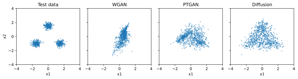
These deliberately short CPU runs show the workflow and its diagnostics, not a tuned performance ranking. Each model gets the same training sample and is scored against independently drawn test rows. Architecture and training costs differ, so an equal step count is not an equal-compute comparison.
Show Python
import numpy as npimport pandas as pdimport torchimport matplotlib.pyplot as pltfrom trex import (TabularTransformer, TabularWGAN, TabularPTGAN, TabularDiffusion, distribution_metrics)torch.set_num_threads(1)rng = np.random.default_rng(812)centers = np.array([[-1.5, -1], [1.5, -1], [0, 1.5]])def draw(n):return centers[rng.integers(3, size=n)] +0.25*rng.normal(size=(n, 2))train, test = draw(800), draw(800)transform = TabularTransformer().fit(train)train_z, test_z = transform.transform(train), transform.transform(test)models = {"WGAN": TabularWGAN(hidden_dims=(32, 32), critic_steps=2, max_steps=350, lr=5e-4, seed=12, device="cpu"),"PTGAN": TabularPTGAN(hidden_dims=(32, 32), max_steps=350, lr=5e-4, seed=12, device="cpu"),"Diffusion": TabularDiffusion(hidden_dims=(48, 48), n_timesteps=200, beta_end=0.05, max_steps=600, seed=12, device="cpu"),}samples, scores = {}, {}for name, model in models.items(): model.fit(train_z) fake_z = model.sample(800).detach().cpu().numpy() samples[name] = transform.inverse_transform(fake_z) scores[name] = distribution_metrics(test_z, fake_z, n_projections=64, seed=9)# Independent real samples give a finite-sample reference, not a zero floor.scores["Real vs real"] = distribution_metrics(test_z, transform.transform(draw(800)), n_projections=64, seed=9)pd.DataFrame(scores).T[["marginal_w1_mean", "corr_frobenius", "sliced_wasserstein"]].round(4)
Figure 1: Held-out data and samples after short training runs. Missing modes and blurred support can be visible even when marginal discrepancies look modest.
Conditional draws and mixed columns
fit(X, context=C) learns a distribution conditional on the supplied context representation. sample(n, context=C_new) requires one context row per requested draw. It does not estimate the marginal law of future contexts; the caller must specify or sample those separately. Avoid extrapolating to unsupported contexts without validation.
TabularTransformer standardizes continuous columns, keeps binary columns on their 0/1 scale, and can round binaries and clip nonnegative columns after inverse transformation. These are post-processing operations, not a mixed discrete/continuous likelihood, and can alter moments or dependence. There is no automatic categorical encoding or missing-value imputation.
What to evaluate
Use training-set scales when comparing columns in different units. Trex’s sliced Wasserstein metric averages empirical 1-Wasserstein distances over random directions and supports unequal sample sizes. Correlation and covariance discrepancies probe dependence, but no finite collection of these scores guarantees useful simulations.
For econometric simulation, additionally examine the actual target: coefficient bias, standard-error coverage, policy ranking, tail events and overlap. Specify causal truth independently when comparing causal estimators; a fitted joint row distribution alone does not define intervention outcomes. Generated rows also do not constitute a privacy guarantee.