Synthetic control and synthetic difference-in-differences

Compare counterfactual paths and understand unit and time weighting.

A treated block in a balanced panel

Arrange outcomes as an N\times T matrix: controls first, treated units last; pre-treatment columns first, post-treatment columns last. N0 and T0 mark the ends of the control and pre-period blocks. These estimators assume a common treatment start and a complete outcome matrix. They are not a staggered-adoption or arbitrary missing-panel interface.

Difference-in-differences subtracts an average control trend. Synthetic control instead forms a weighted combination of donors whose pre-treatment outcomes match the treated unit. Synthetic DID combines unit weights \omega and pre-period weights \lambda:

\hat\tau=\sum_{i,t}\widetilde\omega_i\widetilde\lambda_tY_{it},\qquad \widetilde\omega=(-\omega,\mathbf1/N_1),\quad \widetilde\lambda=(-\lambda,\mathbf1/T_1).

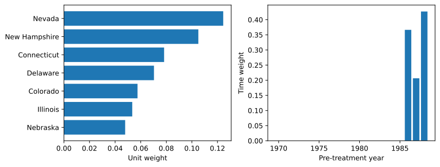
The SDID donor fit allows an intercept: matching the evolution of outcomes does not require matching their level exactly. Time weights compare the controls’ pre-period outcomes to their average post-period outcomes. Ridge regularization and simplex constraints limit unstable extrapolation.

The simplex subproblem

Trex solves subproblems of the form

\min_{w\ge0,\,\mathbf1'w=1}\|Aw-b\|_2^2+n\zeta^2\|w\|_2^2.

With an intercept, it centers the columns and target before the weight fit. The solver is a Frank–Wolfe algorithm, with an optional sparsification and refinement pass. Its stopping rule uses improvement in the objective; it is not a reported KKT/duality-gap certificate. Check stability to maxiter and min_decrease when an optimum lies near a simplex boundary. This is distinct from CrabbyMetrics’ synthetic-control implementation.

Worked example: California Proposition 99

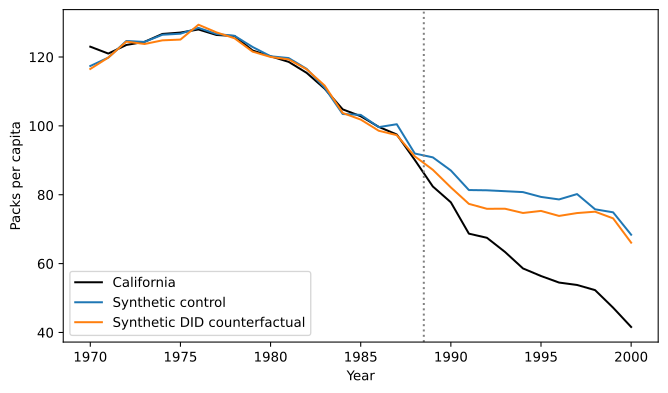
The small cigarette-sales panel is included as a test fixture from the synthdid project; its attribution and license are in tests/data/. No network download is needed to render this example. The outcome is annual packs sold per capita; California’s treatment starts in 1989.

from pathlib import Path
import numpy as np
import pandas as pd
import torch
import matplotlib.pyplot as plt
from trex import SyntheticDID, sc_estimate, did_estimate

torch.set_num_threads(1)
frame = pd.read_csv(Path("../tests/data/california_prop99.csv"), sep=";")
wide = frame.pivot(index="State", columns="Year", values="PacksPerCapita")
states = [s for s in wide.index if s != "California"] + ["California"]
wide = wide.loc[states]
years = wide.columns.to_numpy()
Y = torch.tensor(wide.to_numpy(), dtype=torch.float64)
N0, T0 = len(states)-1, int((years < 1989).sum())
settings = dict(maxiter=10000, min_decrease=1e-5, device="cpu")
sc = sc_estimate(Y, N0, T0, **settings)
sdid = SyntheticDID(**settings).fit(Y, N0, T0).result_
pd.DataFrame({"Effect (packs per capita)": [float(did_estimate(Y, N0, T0)),
                                          float(sc.estimate), float(sdid.estimate)]},
             index=["DID", "SC", "SDID"]).round(3)

	Effect (packs per capita)
DID	-27.349
SC	-19.620
SDID	-15.604

Inspect the path, not only the effect

The SC path is the donor-weighted outcome. For SDID, add the \lambda-weighted pre-period treated-minus-synthetic gap to that path. The mean post-treatment gap then equals the SDID estimate. This adjustment is important: plotting the unadjusted donor path can misrepresent what SDID is comparing.

observed = Y[-1].numpy()
sc_path = (sc.omega @ Y[:N0]).numpy()
sdid_raw = (sdid.omega @ Y[:N0]).numpy()
sdid_path = sdid_raw + float(sdid.lambda_ @ torch.tensor(observed[:T0]-sdid_raw[:T0]))
assert np.isclose((observed[T0:]-sdid_path[T0:]).mean(), float(sdid.estimate))
fig, ax = plt.subplots()
ax.plot(years, observed, color="black", label="California")
ax.plot(years, sc_path, label="Synthetic control")
ax.plot(years, sdid_path, label="Synthetic DID counterfactual")
ax.axvline(1988.5, linestyle=":", color="grey")
ax.set(xlabel="Year", ylabel="Packs per capita"); ax.legend(); plt.show()

Figure 1: Observed California sales and two counterfactual paths. The SDID path includes its weighted pre-period level adjustment.

fig, axes = plt.subplots(1, 2, figsize=(9, 3.5))
weights = sdid.omega.numpy()
top = np.argsort(weights)[-7:]
axes[0].barh(np.array(states[:-1])[top], weights[top])
axes[0].set(xlabel="Unit weight")
axes[1].bar(years[:T0], sdid.lambda_.numpy())
axes[1].set(xlabel="Pre-treatment year", ylabel="Time weight")
fig.tight_layout(); plt.show()

Figure 2: The largest SDID donor weights and its pre-period weights. Concentration is a useful diagnostic, not evidence of identification by itself.

Assumptions, sensitivity, and inference

Good pre-treatment fit is useful evidence about prediction, but does not prove absence of treatment-specific shocks, spillovers, anticipation or donor contamination. Donor selection, intervention timing and outcome definitions remain research decisions. The historical estimate above should not be read as a new causal reanalysis simply because it can be reproduced in Torch.

Examine donor concentration, pre-period residuals, placebo interventions and changes to the donor pool. Select tuning parameters without using treated post-treatment outcomes. Trex exposes point estimates and weights; it does not automatically provide the bootstrap, jackknife or placebo uncertainty procedures used in the SDID literature. Repeated-cell regression standard errors are not a substitute for a justified panel inference procedure.

API: SyntheticDID, sc_estimate, panel_estimates, simplex solver. Background: Arkhangelsky et al. (2021), in references.